Pipeline
Pipelining – MIPS Implementation
The objectives of this module are to discuss the basics of pipelining and discuss the implementation of the MIPS pipeline.
In the previous module, we discussed the drawbacks of a single cycle implementation. We observed that the longest delay determines the clock period and it is not feasible to vary period for different instructions. This violates the design principle of making the common case fast. One way of overcoming this problem is to go in for a pipelined implementation. We shall now discuss the basics of pipelining. Pipelining is a particularly effective way of organizing parallel activity in a computer system. The basic idea is very simple. It is frequently encountered in manufacturing plants, where pipelining is commonly known as an assembly line operation. By laying the production process out in an assembly line, products at various stages can be worked on simultaneously. You must have noticed that in an automobile assembly line, you will find that one car’s chassis will be fitted when some other car’s door is getting fixed and some other car’s body is getting painted. All these are independent activities, taking place in parallel. This process is also referred to as pipelining, because, as in a pipeline, new inputs are accepted at one end and previously accepted inputs appear as outputs at the other end. As yet another real world example, Consider the case of doing a laundry. Assume that Ann, Brian, Cathy and Daveeach have one load of clothes to wash, dry, and fold and that the washer takes 30 minutes, dryer takes 40 minutes and the folder takes 20 minutes. Sequential laundry takes 6 hours for 4 loads. On the other hand, if they learned pipelining, how long would the laundry take? It takes only 3.5 hours for 4 loads! For four loads, you get a Speedup = 6/3.5 = 1.7. If you work the washing machine non-stop, you get a Speedup = 110n/40n + 70 ≈ 3 = number of stages.
To apply the concept of instruction execution in pipeline, it is required to break the instruction execution into different tasks. Each task will be executed in different processing elements of the CPU. As we know that there are two distinct phases of instruction execution: one is instruction fetch and the other one is instruction execution. Therefore, the processor executes a program by fetching and executing instructions, one after another. The cycle time τ of an instruction pipeline is the time needed to advance a set of instructions one stage through the pipeline. The cycle time can be determined as
![]()
where τm = maximum stage delay (delay through the stage which experiences the largest delay) , k = number of stages in the instruction pipeline, d = the time delay of a latch needed to advance signals and data from one stage to the next. Now suppose that n instructions are processed and these instructions are executed one after another. The total time required Tk to execute all n instructions is
![]()
In general, let the instruction execution be divided into five stages as fetch, decode, execute, memory access and write back, denoted by Fi, Di, Ei, Mi and Wi. Execution of a program consists of a sequence of these steps. When the first instruction’s decode happens, the second instruction’s fetch is done. When the pipeline is filled, you see that there are five different activities taking place in parallel. All these activities are overlapped. Five instructions are in progress at any given time. This means that five distinct hardware units are needed. These units must be capable of performing their tasks simultaneously and without interfering with one another. Information is passed from one unit to the next through a storage buffer. As an instruction progresses through the pipeline, all the information needed by the stages downstream must be passed along.
If all stages are balanced, i.e., all take the same time,
If the stages are not balanced, speedup will be less. Observe that the speedup is due to increased throughput and the latency (time for each instruction) does not decrease.
The basic features of pipelining are:
• Pipelining does not help latency of single task, it only helps throughput of entire workload
• Pipeline rate is limited by the slowest pipeline stage
• Multiple tasks operate simultaneously
• It exploits parallelism among instructions in a sequential instruction stream
• Unbalanced lengths of pipe stages reduces speedup
• Time to “fill” pipeline and time to “drain” it reduces speedup
• Ideally the speedup is equal to the number of stages and the CPI is 1
Let us consider the MIPS pipeline with five stages, with one step per stage:
• IF: Instruction fetch from memory
• ID: Instruction decode & register read
• EX: Execute operation or calculate address
• MEM: Access memory operand
• WB: Write result back to register
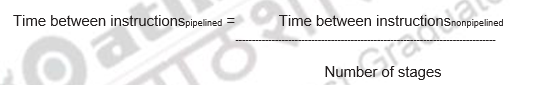
Consider the details given in Figure 10.1. Assume that it takes 100ps for a register read or write and 200ps for all other stages. Let us calculate the speedup obtained by pipelining.
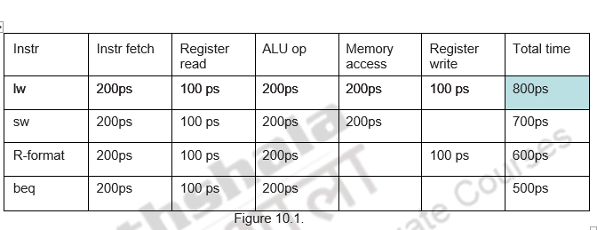
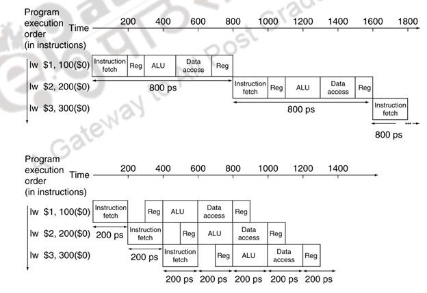
Figure 10.2
For a non pipelined implementation it takes 800ps for each instruction and for a pipelined implementation it takes only 200ps.
Observe that the MIPS ISA is designed in such a way that it is suitable for pipelining.
Figure 10.3 shows the MIPS pipeline implementation.
– All instructions are 32-bits
- Easier to fetch and decode in one cycle
- Comparatively, the x86 ISA: 1- to 17-byte instructions
– Few and regular instruction formats
- Can decode and read registers in one step
– Load/store addressing
- Can calculate address in 3rd stage, access memory in 4th stage
– Alignment of memory operands
- Memory access takes only one cycle
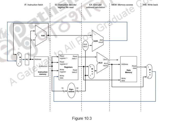
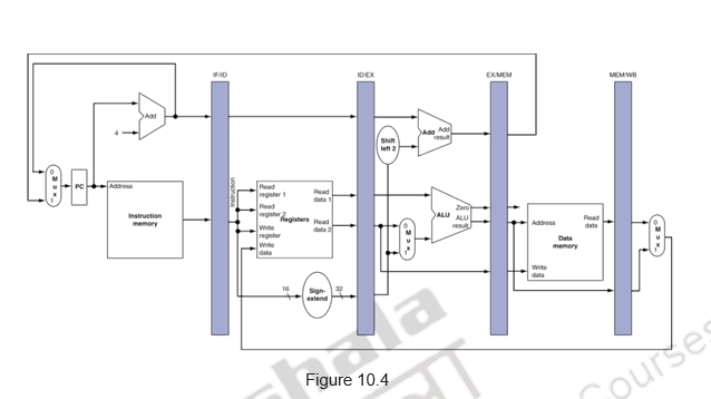
Figure 10.4 shows how buffers are introduced between the stages. This is mandatory. Each stage takes in data from that buffer, processes it and write into the next buffer. Also note that as an instruction moves down the pipeline from one buffer to the next, its relevant information also moves along with it. For example, during clock cycle 4, the information in the buffers is as follows:
- Buffer IF/ID holds instruction I4, which was fetched in cycle 4
- Buffer ID/EX holds the decoded instruction and both the source operands for instruction I3. This is the information produced by the decoding hardware in cycle 3.
- Buffer EX/MEM holds the executed result of I2. The buffer also holds the information needed for the write step of instruction I2. Even though it is not needed by the execution stage, this information must be passed on to the next stage and further down to the Write back stage in the following clock cycle to enable that stage to perform the required Write operation.
- Buffer MEM/WB holds the data fetched from memory (for a load) for I1, and for the arithmetic and logical operations, the results produced by the execution unit and the destination information for instruction I1 are just passed.
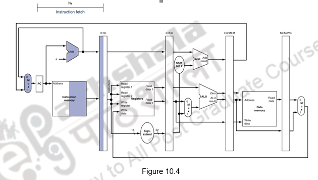
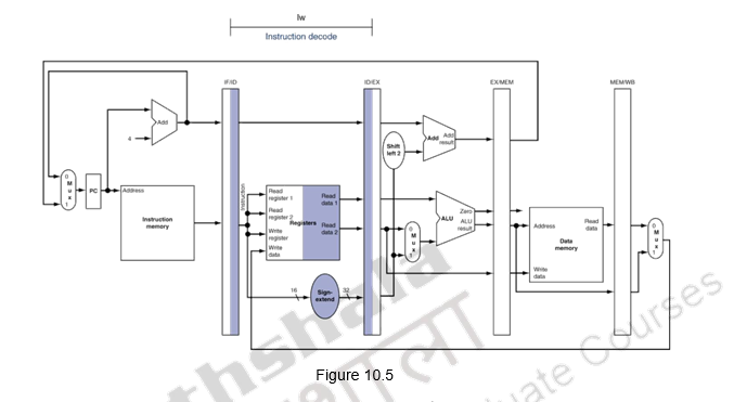
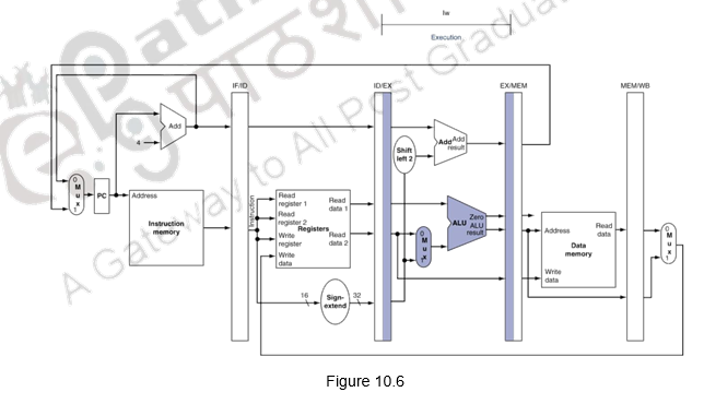
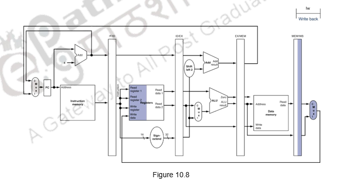
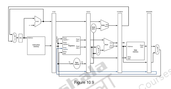
We shall look at the single-clock-cycle diagrams for the load & store instructions of the MIPS ISA. Figure 10.4 shows the instruction fetch for a load / store instruction. Observe that the PC is used to fetch the instruction, it is written into the IF/ID buffer and the PC is incremented by 4. Figure 10.5 shows the next stage of ID. The instruction is decoded, the register file is read and the operands are written into the ID/EX buffer. Note that the entire information of the instruction including the destination register is written into the ID/EX buffer. The highlights in the figure show the resources involved. Figure 10.6 shows the execution stage. The base register’s contents and the sign extended displacement are fed to the ALU, the addition operation is initiated and the ALU calculates the memory address. This effective address is stored in the EX/MEM buffer. Also the destination register’s information is passed from the ID/EX buffer to the EX/MEM buffer. Next, the memory access happens and the read data is written into the MEM/WB buffer. The destination register’s information is passed from the EX/MEM buffer to the MEM/WB buffer. This is illustrated in Figure 10.7. The write back happens in the last stage. The data read from the data memory is written into the destination register specified in the instruction. This is shown in Figure 10.8. The destination register information is passed on from the MEM/WB memory backwards to the register file, along with the data to be written. The datapath is shown in Figure 10.9.

For a store instruction, the effective address calculation is the same as that of load. But when it comes to the memory access stage, store performs a memory write. The effective address is passed on from the execution stage to the memory stage, the data read from the register file is passed from the ID/EX buffer to the EX/MEM buffer and taken from there. The store instruction completes with this memory stage. There is no write back for the store instruction.
While discussing the cycle-by-cycle flow of instructions through the pipelined datapath, we can look at the following options:
- “Single-clock-cycle” pipeline diagram
- Shows pipeline usage in a single cycle
- Highlight resources used
- o “multi-clock-cycle” diagram
- Graph of operation over time
The multi-clock-cycle pipeline diagram showing the resource utilization is given in Figure 10.10. It can be seen that the Instruction memory is used in eth first stage, The register file is used in the second stage, the ALU in the third stage, the data memory in the fourth stage and the register file in the fifth stage again.
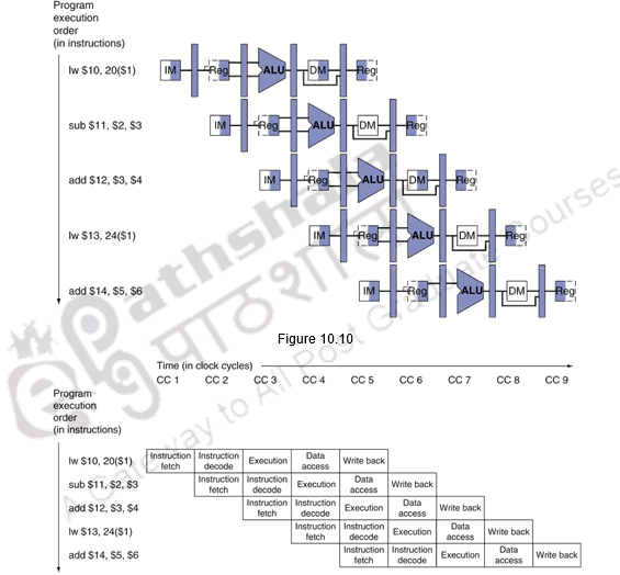
Figure 10.11
The multi-cycle diagram showing the activities happening in each clock cycle is given in Figure 10.11.
Now, having discussed the pipelined implementation of the MIPS architecture, we need to discuss the generation of control signals. The pipelined implementation of MIPS, along with the control signals is given in Figure 10.12.
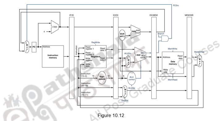
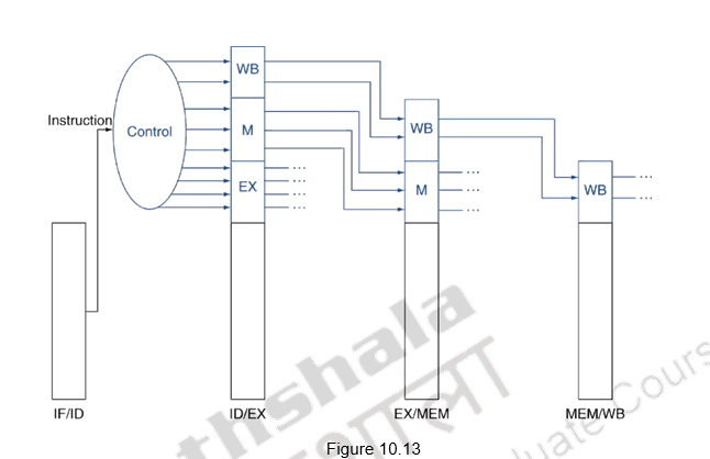
All the control signals indicated are not required at the same time. Different control signals are required at different stages of the pipeline. But the decision about the generation of the various control signals is done at the second stage, when the instruction is decoded. Therefore, just as the data flows from one stage to another as the instruction moves from one stage to another, the control signals also pass on from one buffer to another and are utilized at the appropriate instants. This is shown in Figure 10.13. The control signals for the execution stage are used in that stage. The control signals needed for the memory stage and the write back stage move along with that instruction to the next stage. The memory related control signals are used in the next stage, whereas, the write back related control signals move from there to the next stage and used when the instruction performs the write back operation.
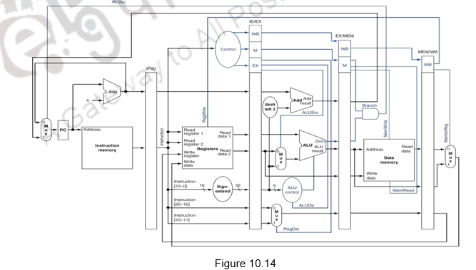
The complete pipeline implementation, along with the control signals used at the various stages is given in Figure 10.14.
To summarize, we have discussed the basics of pipelining in this module. We have made the following observations about pipelining.
- Pipelining is overlapped execution of instructions
- Latency is the same, but throughput improves
- Pipeline rate limited by slowest pipeline stage
- Potential speedup = Number of pipe stages
We have discussed about the implementation of pipelining in the MIPS architecture. We have shown the implementation of the various buffers, the data flow and the control flow for a pipelined implementation of the MIPS architecture.
Web Links / Supporting Materials
- Computer Organization and Design – The Hardware / Software Interface, David A. Patterson and John L. Hennessy, 4th.Edition, Morgan Kaufmann, Elsevier, 2009.
- Computer Organization, Carl Hamacher, Zvonko Vranesic and Safwat Zaky, 5th.Edition, McGraw- Hill Higher Education, 2011.
Pipeline Hazards
The objectives of this module are to discuss the various hazards associated with pipelining.
We discussed the basics of pipelining and the MIPS pipeline implementation in the previous module. We made the following observations about pipelining:
- Pipelining doesn’t help latency of single task, it helps throughput of entire workload
- Pipeline rate limited by slowest pipeline stage o Multiple tasks operating simultaneously
- Potential speedup = Number of pipe stages
- Unbalanced lengths of pipe stages reduces speedup
- Time to “fill” pipeline and time to “drain” it reduces speedup o Unbalanced lengths of pipe stages reduces speedup
- Execute billions of instructions, so throughput is what matters o Data path design – Ideally we expect a CPI value of 1
- What is desirable in instruction sets for pipelining?
- Variable length instructions vs. all instructions same length?
- Memory operands part of any operation vs. memory operands only in loads or stores?
- Register operand many places in instruction format vs. registers located in same place?
Ideally we expect a CPI value of 1 and a speedup equal to the number of stages in the pipeline. But, there are a number of factors that limit this. The problems that occur in the pipeline are called hazards. Hazards that arise in the pipeline prevent the next instruction from executing during its designated clock cycle. There are three types of hazards:
- Structural hazards: Hardware cannot support certain combinations of instructions (two instructions in the pipeline require the same resource).
- Data hazards: Instruction depends on result of prior instruction still in the pipeline
- Control hazards: Caused by delay between the fetching of instructions and decisions about changes in control flow (branches and jumps).
Structural hazards arise because there is not enough duplication of resources.
Resolving structural hazards:
- Solution 1: Wait
o Must detect the hazard
o Must have mechanism to stall
o Low cost and simple
o Increases CPI
o Used for rare cases
- Solution 2: Throw more hardware at the problem
o Pipeline hardware resource
§ useful for multi-cycle resources
§ good performance
§ sometimes complex e.g., RAM
o Replicate resource
§ good performance
§ increases cost (+ maybe interconnect delay)
§ useful for cheap or divisible resource
Figure 11.1 shows one possibility of a structural hazard in the MIPS pipeline. Instruction 3 is accessing memory for an instruction fetch and instruction 1 is accessing memory for a data access (load/store). These two are conflicting requirements and gives rise to a hazard. We should either stall one of the operations as shown in Figure 11.2, or have two separate memories for code and data. Structural hazards will have to handled at the design time itself.
Next, we shall discuss about data dependences and the associated hazards. There are two types of data dependence – true data dependences and name dependences.
• An instruction j is data dependent on instruction i if either of the following holds:
– Instruction i produces a result that may be used by instruction j, or
– Instruction j is data dependent on instruction k, and instruction k is data dependent on instruction i
• A name dependence occurs when two instructions use the same register or memory location, called a name, but there is no flow of data between the instructions associated with that name
– Two types of name dependences between an instruction i that precedes instruction j in program order:
– An antidependence between instruction i and instruction j occurs when instruction j writes a register or memory location that instruction i reads. The original ordering must be preserved.
– An output dependence occurs when instruction i and instruction j write the same register or memory location. The ordering between the instructions must be preserved.
– Since this is not a true dependence, renaming can be more easily done for register operands, where it is called register renaming
– Register renaming can be done either statically by a compiler or dynamically by the hardware
Last of all, we discuss control dependences. Control dependences determine the ordering of an instruction with respect to a branch instruction so that an instruction i is executed in correct program order. There are two general constraints imposed by control dependences:
– An instruction that is control dependent on its branch cannot be moved before the branch so that its execution is no longer controlled by the branch.
– An instruction that is not control dependent on its branch cannot be moved after the branch so that its execution is controlled by the branch.
Having introduced the various types of data dependences and control dependence, let us discuss how these dependences cause problems in the pipeline. Dependences are properties of programs and whether the dependences turn out to be hazards and cause stalls in the pipeline are properties of the pipeline organization.
Data hazards may be classified as one of three types, depending on the order of read and write accesses in the instructions:
- RAW (Read After Write)
- Corresponds to a true data dependence
- Program order must be preserved
- This hazard results from an actual need for communication
- Considering two instructions i and j, instruction j reads the data before i writes it
i: ADD R1, R2, R3
j: SUB R4, R1, R3
Add modifies R1 and then Sub should read it. If this order is changed, there is a RAW hazard
- WAW (Write After Write)
- Corresponds to an output dependence
- Occurs when there are multiple writes or a short integer pipeline and a longer floating-point pipeline or when an instruction proceeds when a previous instruction is stalled WAW (write after write)
- This is caused by a name dependence. There is no actual data transfer. It is the same name that causes the problem
- Considering two instructions i and j, instruction j should write after instruction i has written the data
i: SUB R1, R4, R3
j: ADD R1, R2, R3
Instruction i has to modify register r1 first, and then j has to modify it. Otherwise, there is a WAW hazard. There is a problem because of R1. If some other register had been used, there will not be a problem
- Solution is register renaming, that is, use some other register. The hardware can do the renaming or the compiler can do the renaming
- WAR (Write After Read)
- Arises from an anti dependence
- Cannot occur in most static issue pipelines
- Occurs either when there are early writes and late reads, or when instructions are re-ordered
- There is no actual data transfer. It is the same name that causes the problem
- Considering two instructions i and j, instruction j should write after instruction i has read the data.
i: SUB R4, R1, R3
j: ADD R1, R2, R3
Instruction i has to read register r1 first, and then j has to modify it. Otherwise, there is a WAR hazard. There is a problem because of R1. If some other register had been used, there will not be a problem
• Solution is register renaming, that is, use some other register. The hardware can do the renaming or the compiler can do the renaming
Figure 11.3 gives a situation of having true data dependences. The use of the result of the ADD instruction in the next three instructions causes a hazard, since the register is not written until after those instructions read it. The write back for the ADD instruction happens only in the fifth clock cycle, whereas the next three instructions read the register values before that, and hence will read the wrong data. This gives rise to RAW hazards.
A control hazard is when we need to find the destination of a branch, and can’t fetch any new instructions until we know that destination. Figure 11.4 illustrates a control hazard. The first instruction is a branch and it gets resolved only in the fourth clock cycle. So, the next three instructions fetched may be correct, or wrong, depending on the outcome of the branch. This is an example of a control hazard.
Now, having discussed the various dependences and the hazards that they might lead to, we shall see what are the hazards that can happen in our simple MIPS pipeline.
- Structural hazard
- Conflict for use of a resource
• In MIPS pipeline with a single memory
– Load/store requires data access
– Instruction fetch would have to stall for that cycle
• Would cause a pipeline “bubble”
• Hence, pipelined datapaths require separate instruction/data memories or separate instruction/data caches
- RAW hazards – can happen in any architecture
- WAR hazards – Can’t happen in MIPS 5 stage pipeline because all instructions take 5 stages, and reads are always in stage 2, and writes are always in stage 5
- WAW hazards – Can’t happen in MIPS 5 stage pipeline because all instructions take 5 stages, and writes are always in stage 5
- Control hazards
- Can happen
- The penalty depends on when the branch is resolved – in the second clock cycle or the third clock cycle
- More aggressive implementations resolve the branch in the second clock cycle itself, leading to one clock cycle penalty
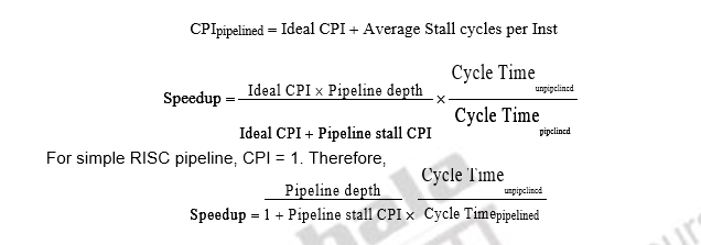
Let us look at the speedup equation with stalls and look at an example problem.
CPIpipelined = Ideal CPI + Average Stall cycles per Inst
Let us assume we want to compare the performance of two machines. Which machine is faster?
- Machine A: Dual ported memory – so there are no memory stalls
- Machine B: Single ported memory, but its pipelined implementation has a 1.05 times faster clock rate
Assume:
- Ideal CPI = 1 for both
- Loads are 40% of instructions executed
SpeedupA = Pipeline Depth/(1+0) x(clockunpipe/clockpipe)
= Pipeline Depth
SpeedupB = Pipeline Depth/(1 + 0.4 x 1) x (clockunpipe/(clockunpipe / 1.05)
= (Pipeline Depth/1.4) x 1.05
= 75 x Pipeline Depth
SpeedupA / SpeedupB = Pipeline Depth / (0.75 x Pipeline Depth) = 1.33 Machine A is 1.33 times faster.
To summarize, we have discussed the various hazards that might occur in a pipeline. Structural hazards happen because there are not enough duplication of resources and they have to be handled at design time itself. Data hazards happen because of true data dependences and name dependences. Control hazards are caused by branches. The solutions for all these hazards will be discussed in the subsequent modules.
Web Links / Supporting Materials
- Computer Organization and Design – The Hardware / Software Interface, David A. Patterson and John L. Hennessy, 4th.Edition, Morgan Kaufmann, Elsevier, 2009.
- Computer Organization, Carl Hamacher, Zvonko Vranesic and Safwat Zaky, 5th.Edition, McGraw- Hill Higher Education, 2011.
Handling Data Hazards
The objectives of this module are to discuss how data hazards are handled in general and also in the MIPS architecture.
We have already discussed in the previous module that true data dependences give rise to RAW hazards and name dependences (antidependence and output dependence) give rise to WAR hazards and WAW hazards, respectively.
Figure 12.1 gives a situation of having true data dependences. The use of the result of the ADD instruction in the next three instructions causes a hazard, since the register is not written until after those instructions read it. The write back for the ADD instruction happens only in the fifth clock cycle, whereas the next three instructions read the register values before that, and hence will read the wrong data. This gives rise to RAW hazards.
One effective solution to handle true data dependences is forwarding. Forwarding is the concept of making data available to the input of the ALU for subsequent instructions, even though the generating instruction hasn’t gotten to WB in order to write the memory or registers. This is also called short circuiting or by passing. This is illustrated in Figure 12.2.
The first instruction has finished execution and the result has been written into the EX/MEM buffer. So, during the fourth clock cycle, when the second instruction, SUB needs data, this can be forwarded from the EX/MEM buffer to the input of the ALU. Similarly, for the next AND instruction, the result of the first instruction is now available in the MEM/WB buffer and can be forwarded from there. For the OR instruction, the result is written into the register file during the first half of the clock cycle and the data from there is read during the second half. So, this instruction has no problem. In short, data will have to be forwarded from either the EX/MEM buffer or the MEM/WB buffer.
Figure 12.3 shows the hardware changes required to support forwarding. The inputs to the ALU have increased. The multiplexors will have to be expanded, in order to accommodate the additional inputs from the two buffers.
Figure 12.4 shows a case where the first instruction is a load and the data becomes available only after the fourth clock cycle. So, forwarding will not help and the second instruction will anyway have a stall of one cycle. For the next instruction, AND, data is forwarded from the MEM/WB buffer. There are thus instances where stalls may occur even with forwarding. However, forwarding is helpful in minimizing hazards and sometimes in totally eliminating them.
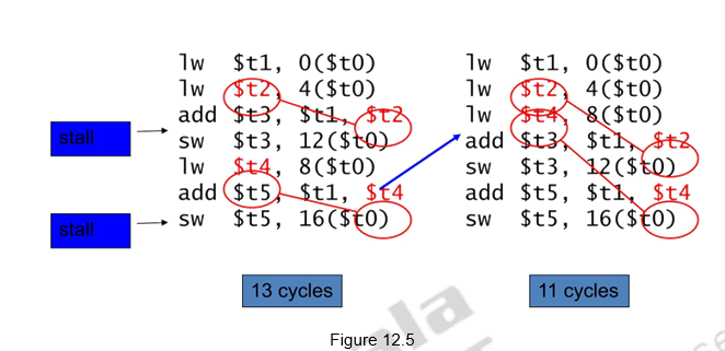
The other method of avoiding / minimizing stalls due to true data dependences is to reorder the code – separate the dependent instructions. This is illustrated in Figure 12.5. The snippet shown calculates A = B + E; C = B + F; The dependent instruction after the load can be reordered to avoid use of load result in the next instruction. This reordering has helped in reducing the number of clock cycles for execution from 13 to 11. Two stalls have been avoided.
Based on the discussion given earlier, we can identify the two pairs of hazard conditions as:
1a. EX/MEM.RegisterRd = ID/EX.RegisterRs
1b. EX/MEM.RegisterRd = ID/EX.RegisterRt
2a. MEM/WB.RegisterRd = ID/EX.RegisterRs
2b. MEM/WB.RegisterRd = ID/EX.RegisterRt
The notation used here is as follows: The first part of the name, to the left of the period, is the name of the pipeline register and the second part is the name of the field in that register. For example, “ID/EX.RegisterRs” refers to the number of one register whose value is found in the pipeline register ID/EX; that is, the one from the first read port of the register file. We shall discuss the various hazards based on the following sequence of instructions.

The first hazard in the sequence is on register 2,3 and the first read operand of and 2,2
The sub-or is a type 2b hazard:
MEM/WB.RegisterRd = ID/EX.RegisterRt = $2
The two dependences on sub-add are not hazards because the register file supplies the proper data during the ID stage of add. There is no data hazard between sub and sw because sw reads 2. However, as some instructions do not write into the register file, this rule has to be modified. Otherwise, sometimes it would forward when it was unnecessary. One solution is simply to check to see if the RegWrite signal will be active. Examining the WB control field of the pipeline register during the EX and MEM stages determines if RegWrite is asserted or not. Also, MIPS requires that every use of 0 as its destination (for example, sll 1, 2), we want to avoid forwarding its possibly nonzero result value. The conditions above thus work properly as long as we add EX/MEM.RegisterRd ≠ 0 to the first hazard condition and MEM/WB.RegisterRd ≠ 0 to the second.
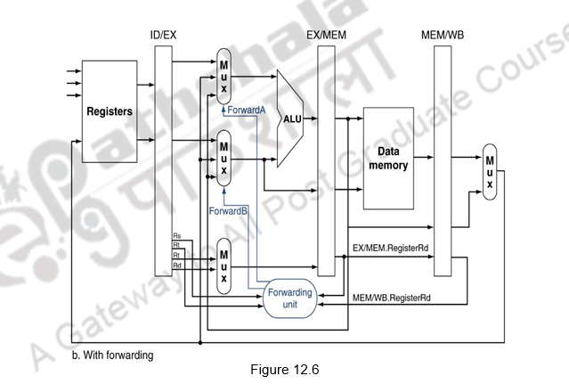
Figure 12.6 shows the forwarding paths added to the MIPS pipeline. The ForwardA and ForwardB are the additional control signals added. These control signals take on a value of 00, 10 or 01, depending on whether the multiplexor will pass on the data from the ID/EX, EX/MEM or MEM/WB buffers, respectively.
The conditions for detecting hazards and the control signals to resolve them are as follows:
1. EX hazard:
if (EX/MEM.RegWrite
and (EX/MEM.RegisterRd _ 0)
and (EX/MEM.RegisterRd = ID/EX.RegisterRs)) ForwardA = 10
if (EX/MEM.RegWrite
and (EX/MEM.RegisterRd _ 0)
and (EX/MEM.RegisterRd = ID/EX.RegisterRt)) ForwardB = 10
This case forwards the result from the previous instruction to either input of the ALU. If the previous instruction is going to write to the register file and the write register number matches the read register number of ALU inputs A or B, provided it is not register 0, then direct the multiplexor to pick the value instead from the pipeline register EX/MEM.
2. MEM hazard:
if (MEM/WB.RegWrite
and (MEM/WB.RegisterRd _ 0)
and (MEM/WB.RegisterRd = ID/EX.RegisterRs)) ForwardA = 01
if (MEM/WB.RegWrite
and (MEM/WB.RegisterRd _ 0)
and (MEM/WB.RegisterRd = ID/EX.RegisterRt)) ForwardB = 01
As mentioned above, there is no hazard in the WB stage because we assume that the register file supplies the correct result if the instruction in the ID stage reads the same register written by the instruction in the WB stage. Such a register file performs another form of forwarding, but it occurs within the register file.
Another complication is the potential data hazards between the result of the instruction in the WB stage, the result of the instruction in the MEM stage, and the source operand of the instruction in the ALU stage. For example, when summing a vector of numbers in a single register, a sequence of instructions will all read and write to the same register as indicated below:
add 1,$2
add 1,$3
add 1,$4
. . .
In this case, the result is forwarded from the MEM stage because the result in the MEM stage is the more recent result. Thus the control for the MEM hazard would be (with the additions highlighted)
if (MEM/WB.RegWrite
and (MEM/WB.RegisterRd _ 0)
and (EX/MEM.RegisterRd _ ID/EX.RegisterRs)
and (MEM/WB.RegisterRd = ID/EX.RegisterRs)) ForwardA = 01
if (MEM/WB.RegWrite
and (MEM/WB.RegisterRd _ 0)
and (EX/MEM.RegisterRd _ ID/EX.RegisterRt)
and (MEM/WB.RegisterRd = ID/EX.RegisterRt)) ForwardB = 01
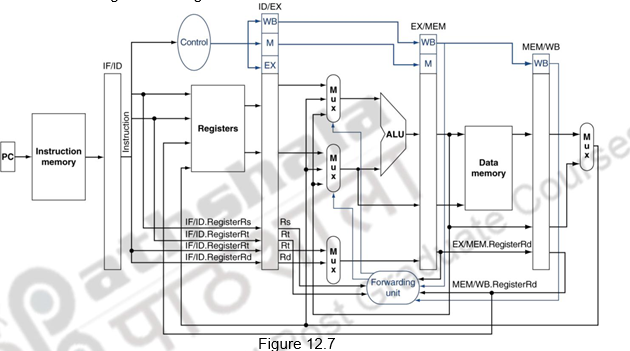
Figure 12.7 shows the datapath modified to resolve hazards via forwarding. Compared with the datapath already shown, the additions are the multiplexors to the inputs to the ALU.
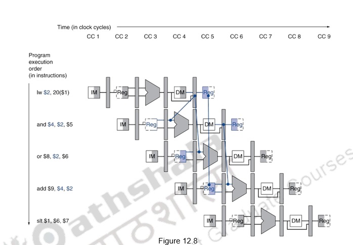
As we already discussed, one case where forwarding cannot help eliminate hazards is when an instruction tries to read a register following a load instruction that writes the same register. This is illustrated in Figure 12.8. The data is still being read from memory in clock cycle 4 while the ALU is performing the operation for the following instruction. Something must stall the pipeline for the combination of load followed by an instruction that reads its result. Hence, in addition to a forwarding unit, we need a hazard detection unit. It operates during the ID stage so that it can insert the stall between the load and its use. Checking for load instructions, the control for the hazard detection unit is this single condition:
if (ID/EX.MemRead and
((ID/EX.RegisterRt = IF/ID.RegisterRs) or
(ID/EX.RegisterRt = IF/ID.RegisterRt)))
stall the pipeline
The first line tests to see if the instruction is a load. The only instruction that reads data memory is a load. The next two lines check to see if the destination register field of the load in the EX stage matches either source register of the instruction in the ID stage. If the condition holds, the instruction stalls 1 clock cycle. After this 1-cycle stall, the forwarding logic can handle the dependence and execution proceeds. If there were no forwarding, then the instructions would need another stall cycle.
If the instruction in the ID stage is stalled, then the instruction in the IF stage must also be stalled; otherwise, we would lose the fetched instruction. Preventing these two instructions from making progress is accomplished simply by preventing the PC register and the IF/ID pipeline register from changing. Provided these registers are preserved, the instruction in the IF stage will continue to be read using the same PC, and the registers in the ID stage will continue to be read using the same instruction fields in the IF/ID pipeline register. The back half of the pipeline starting with the EX stage must be executing instructions that have no effect. This is done by executing nops. Deasserting all the nine control signals (setting them to 0) in the EX, MEM, and WB stages will create a “do nothing” or nop instruction. By identifying the hazard in the ID stage, we can insert a bubble into the pipeline by changing the EX, MEM, and WB control fields of the ID/EX pipeline register to 0. These control values are percolated forward at each clock cycle with the proper effect – no registers or memories are written if the control values are all 0.
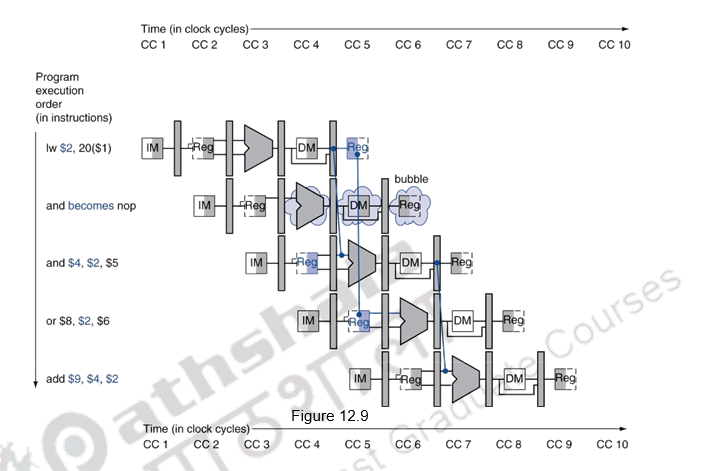
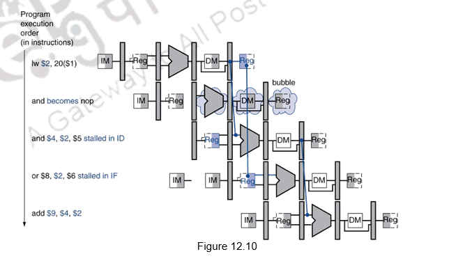
Figures 12.9 and 12.10 show what really happens in the hardware: the pipeline execution slot associated with the AND instruction is turned into a NOP and all instructions beginning with the AND instruction are delayed one cycle. The hazard forces the AND and OR instructions to repeat in clock cycle 4 what they did in clock cycle 3: and reads registers and decodes, and OR is refetched from instruction memory. Such repeated work is what a stall looks like, but its effect is to stretch the time of the AND and OR instructions and delay the fetch of the ADD instruction. Like an air bubble in a water pipe, a stall bubble delays everything behind it and proceeds down the instruction pipe one stage each cycle until it exits at the end.
Figure 12.11 highlights the pipeline connections for both the hazard detection unit and the forwarding unit
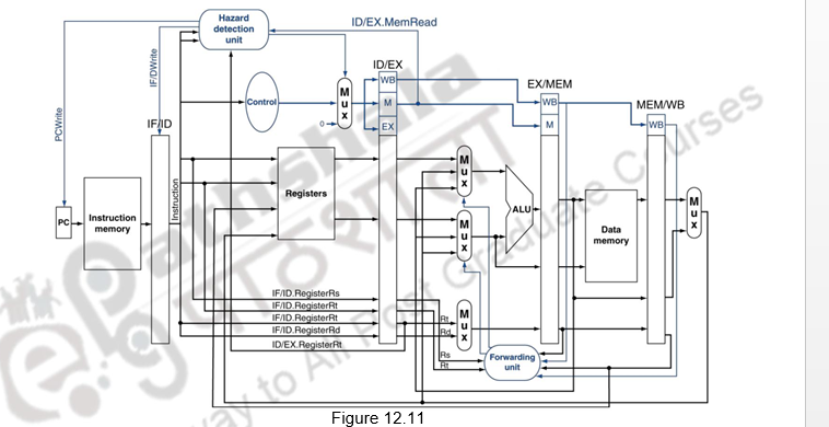
As discussed before, the forwarding unit controls the ALU multiplexors to replace the value from a general-purpose register with the value from the proper pipeline register. The hazard detection unit controls the writing of the PC and IF/ID registers plus the multiplexor that chooses between the real control values and all 0s. The hazard detection unit stalls and deasserts the control fields if the load-use hazard test is true.
It should be noted that stalls reduce performance, but are required to get correct results. Also remember that the compiler can arrange code to avoid hazards and stalls and it requires knowledge of the pipeline structure to do this. For the other types of data hazards, viz. WAR and WAW hazards where there is no true sharing of data, they can be resolved by register renaming, which can be handled by the hardware or the compiler. This renaming can happen with memory operands also, which is more difficult to handle, because it is difficult to resolve the ambiguity associated with memory operands.
To summarize, in this module we have discussed about how data hazards can be handled by forwarding. This technique requires needs extra hardware paths and control. All cases may not be handled and stalls may be necessary. To avoid WAR and WAW hazards, register renaming by software or hardware can be done. RAW hazards can also be handled by reorganization of code, either by software or hardware. The hardware reorganization of code during execution will be discussed in later modules.
Web Links / Supporting Materials
- Computer Organization and Design – The Hardware / Software Interface, David A. Patterson and John L. Hennessy, 4th.Edition, Morgan Kaufmann, Elsevier, 2009.
- Computer Organization, Carl Hamacher, Zvonko Vranesic and Safwat Zaky, 5th.Edition, McGraw- Hill Higher Education, 2011.
Handling Control Hazards
The objectives of this module are to discuss how to handle control hazards, to differentiate between static and dynamic branch prediction and to study the concept of delayed branching.
A branch in a sequence of instructions causes a problem. An instruction must be fetched at every clock cycle to sustain the pipeline. However, until the branch is resolved, we will not know where to fetch the next instruction from and this causes a problem. This delay in determining the proper instruction to fetch is called a control hazard or branch hazard, in contrast to the data hazards we examined in the previous modules. Control hazards are caused by control dependences. An instruction that is control dependent on a branch cannot be moved in front of the branch, so that the branch no longer controls it and an instruction that is not control dependent on a branch cannot be moved after the branch so that the branch controls it. This will give rise to control hazards.
The two major issues related to control dependences are exception behavior and handling and preservation of data flow. Preserving exception behavior requires that any changes in instruction execution order must not change how exceptions are raised in program. That is, no new exceptions should be generated.
| • Example: | |
| ADD | R2,R3,R4 |
| BEQZ | R2,L1 |
| LD | R1,0(R2) |
| L1: |
What will happen with moving LD before BEQZ? This may lead to memory protection violation. The branch instruction is a guarding branch that checks for an address zero and jumps to L1. If this is moved ahead, then an additional exception will be raised. Data flow is the actual flow of data values among instructions that produce results and those that consume them. Branches make flow dynamic and determine which instruction is the supplier of data
• Example:
| DSUBU | R1,R5,R6 |
| L:… | |
| OR | R7,R1,R8 |
The instruction OR depends on DADDU or DSUBU? We must ensure that we preserve data flow on execution.
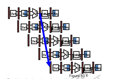
The general rule to reduce branch penalties is to resolve branches as early as possible. In the MIPS pipeline, the comparison of registers and target address calculation is normally done at the execution stage. This gives rise to three clock cycles penalty. This is indicated in Figure 13.1. If we do a more aggressive implementation by adding hardware to resolve the branch in the ID stage, the penalty can be reduced.
Resolving the branch earlier requires two actions to occur – computing the branch target address and evaluating the branch decision early. The easy part of this change is to move up the branch address calculation. We already have the PC value and the immediate field in the IF/ID pipeline register, so we just move the branch adder from the EX stage to the ID stage; of course, the branch target address calculation will be performed for all instructions, but only used when needed. The harder part is the branch decision itself. For branch equal, we would compare the two registers read during the ID stage to see if they are equal. Equality can be tested by first exclusive ORing their respective bits and then ORing all the results. Moving the branch test to the ID stage also implies additional forwarding and hazard detection hardware, since a branch dependent on a result still in the pipeline must still work properly with this optimization. For example, to implement branch-on-equal (and its inverse), we will need to forward results to the equality test logic that operates during ID. There are two complicating factors:
- During ID, we must decode the instruction, decide whether a bypass to the equality unit is needed, and complete the equality comparison so that if the instruction is a branch, we can set the PC to the branch target address. Forwarding for the operands of branches was formerly handled by the ALU forwarding logic, but the introduction of the equality test unit in ID will require new forwarding logic. Note that the bypassed source operands of a branch can come from either the ALU/MEM or MEM/WB pipeline latches.
- Because the values in a branch comparison are needed during ID but may be produced later in time, it is possible that a data hazard can occur and a stall will be needed. For example, if an ALU instruction immediately preceding a branch produces one of the operands for the comparison in the branch, a stall will be required, since the EX stage for the ALU instruction will occur after the ID cycle of the branch.
Despite these difficulties, moving the branch execution to the ID stage is an improvement since it reduces the penalty of a branch to only one instruction if the branch is taken, namely, the one currently being fetched.
There are basically two ways of handling control hazards:
1. Stall until the branch outcome is known or perform the fetch again
2. Predict the behavior of branches
a. Static prediction by the compiler
b. Dynamic prediction by the hardware
The first option of stalling the pipeline till the branch is resolved, or fetching again from the resolved address leads to too much of penalty. Branches are very frequent and not handling them effectively brings down the performance. We are also violating the principle of “Make common cases fast”.
The second option is predicting about the behavior of branches. Branch Prediction is the ability to make an educated guess about which way a branch will go – will the branch be taken or not. First of all, we shall discuss about static prediction done by the compiler. This is based on typical branch behavior. For example, for loop and if-statement branches, we can predict that backward branches will be taken and forward branches will not be taken. So, there are primarily three methods adopted. They are:
– Predict not taken approach
• Assume that the branch is not taken, i.e. the condition will not evaluate to be true
– Predict taken approach
• Assume that the branch is taken, i.e. the condition will evaluate to be true
– Delayed branching
• A more effective solution
In the predict not taken approach, treat every branch as “not taken”. Remember that the registers are read during ID, and we also perform an equality test to decide whether to branch or not. We simply load in the next instruction (PC+4) and continue. The complexity arises when the branch evaluates to be true and we end up needing to actually take the branch. In such a case, the pipeline is cleared of any code loaded from the “not-taken” path, and the execution continues.
In the predict-taken approach, we assume that the branch is always taken. This method will work for processors that have the target address computed in time for the IF stage of the next instruction so there is no delay, and the condition alone may not be evaluated. This will not work for the MIPS architecture with a 5-stage pipeline. Here, the branch target is computed during the ID cycle or later and the condition is also evaluated in the same clock cycle.
The third approach is the delayed branching approach. In this case, an instruction that is useful and not dependent on whether the branch is taken or not is inserted into the pipeline. It is the job of the compiler to determine the delayed branch instructions. The slots filled up by instructions which may or may not get executed, depending on the outcome of the branch, are called the branch delay slots. The compiler has to fill these slots with useful/independent instructions. It is easier for the compiler if there are less number of delay slots.
There are three different ways of introducing instructions in the delay slots:
• Before branch instruction
• From the target address: only valuable when branch taken
• From fall through: only valuable when branch is not taken
• Cancelling branches allow more slots to be filled
Figure 13.2 shows the three different ways of filling in instructions in the branch delay slots.
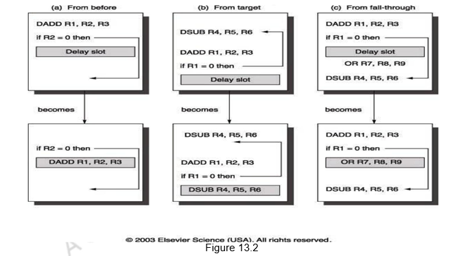
When the first choice is taken, the branch must not depend on the rescheduled instructions and there will always be performance improvement, irrespective of which way the branch goes. When instructions are picked from the target path, the compiler predicts that the branch is going to take. It must be alright to execute rescheduled instructions even if the branch is not taken. That is, the work may be wasted, but the program will still execute correctly. This may need duplication of instructions. There will be improvement in performance only when the branch is taken. When the branch is not taken, the extra instructions may increase the code size. When instructions are picked from the fall through path, the compiler predicts that the branch is not going to take. It must be alright to execute rescheduled instructions even if the branch is taken. This may lead to improvement in performance only if the branch is not taken. The extra instructions added as compensatory code may be an overhead.
The limitations on delayed-branch scheduling arise from (1) the restrictions on the instructions that are scheduled into the delay slots and (2) our ability to predict at compile time whether a branch is likely to be taken or not. If the compiler is not able to find useful instructions, it may fill up the slots with nops, which is not a good option.
To improve the ability of the compiler to fill branch delay slots, most processors with conditional branches have introduced a cancelling or nullifying branch. In a cancelling branch, the instruction includes the direction that the branch was predicted. When the branch behaves as predicted, the instruction in the branch delay slot is simply executed as it would normally be with a delayed branch. When the branch is incorrectly predicted, the instruction in the branch delay slot is simply turned into a no-op. Examples of such branches are Cancel-if-taken or Cancel-if-not-taken branches. In such cases, the compiler need not be too conservative in filling the branch delay slots, because it knows that the hardware will cancel the instruction if the branch behavior goes against the prediction.
The pipeline speedup is given by
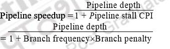
Let us look at an example to calculate the speedup, given the following:
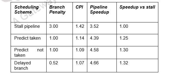
14% Conditional & Unconditional, 65% Taken; 52% Delay slots not usefully filled. The details for the various schemes are provided in the table below.
• Stall: 1+.14(branches)*3(cycle stall)
• Taken: 1+.14(branches)*(.65(taken)*1(delay to find address)+.35(not taken)*1(penalty))
• Not taken: 1+.14*(.65(taken)*1+[.35(not taken)*0])
• Delayed: 1+.14*(.52(not usefully filled)*1)
Other example problems:
Given an application where 20% of the instructions executed are conditional branches and 59% of those are taken. For the MIPS 5-stage pipeline, what speedup will be achieved using a scheme where all branches are predicted as taken over a scheme with no branch prediction (i.e. branches will always incur a 1 cycle penalty)? Ignore all other stalls.
• CPI with no branch prediction
= 0.8 x 1 + 0.2 x 2 = 1.2
• CPI with branch prediction
= 0.8 x 1 + 0.2 x 0.59 x 1 + 0.2 x 0.41 x 2 = 1.082
• Speed up = 1.2 / 1.082 = 1.109
We want to compare the performance of two machines. Which machine is faster?
• Machine A: Dual ported memory – so there are no memory stalls
• Machine B: Single ported memory, but its pipelined implementation has a 1.05 times faster clock rate
Assume:
• Ideal CPI = 1 for both
• Loads are 40% of instructions executed SpeedUpA
= Pipeline Depth/(1 + 0) x (clockunpipe/clockpipe)
= Pipeline Depth
SpeedUpB
- = Pipeline Depth/(1 + 0.4 x 1) x (clockunpipe/(clockunpipe / 1.05)
- = (Pipeline Depth/1.4) x 1.05
- = 75 x Pipeline Depth
SpeedUpA / SpeedUpB
- = Pipeline Depth / (0.75 x Pipeline Depth) = 1.33 Machine A is 1.33 times faster
To summarize, we have discussed about control hazards that arise due to control dependences caused by branches. Branches are very frequent and so have to be handled properly. There are different ways of handling branch hazards. The pipeline can be stalled, but that is not an effective way to handle branches. We discussed the predict taken, predict not taken and delayed branching techniques to handle branch hazards. All these are static techniques. We will discuss further on branch hazards in the next module.
Web Links / Supporting Materials
- Computer Organization and Design – The Hardware / Software Interface, David A. Patterson and John L. Hennessy, 4th.Edition, Morgan Kaufmann, Elsevier, 2009.
- Computer Organization, Carl Hamacher, Zvonko Vranesic and Safwat Zaky, 5th.Edition, McGraw- Hill Higher Education, 2011.
Dynamic Branch Prediction
The objectives of this module are to discuss how control hazards are handled in the MIPS architecture and to look at more realistic branch predictors.
In the previous module, we discussed about the basics of control hazards and discussed about how the compiler handles control hazards. We have seen that longer pipelines can’t readily determine the branch outcome early and the stall penalty becomes unacceptable in such cases. As far as the MIPS pipeline is concerned, we can predict branches as not taken and fetch instructions after the branch, with no delay. Figure 14.1 shows the predict not taken approach, when the prediction is correct and when the prediction is wrong. When the prediction is right, that is, when the branch is not taken, there is no penalty to be paid. On the other hand, when the prediction is wrong, one bubble is created and the next instruction is fetched from the target address. Here, we assume that the branch is resolved in the IF stage itself.
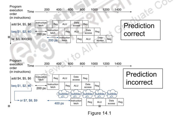
Let us consider the following sequence of operations.
| 36 | sub | 4, 1, 3, 7 # PC-relative branch to 40 + 4 + 7 * 4 = 72</td></tr><tr><td>44</td><td>and</td><td>12, 5 |
| 48 | or | 2, $6 |
| 52 | add | 4, 15, 7 |
| . . . | ||
| 72 | lw | 7) |
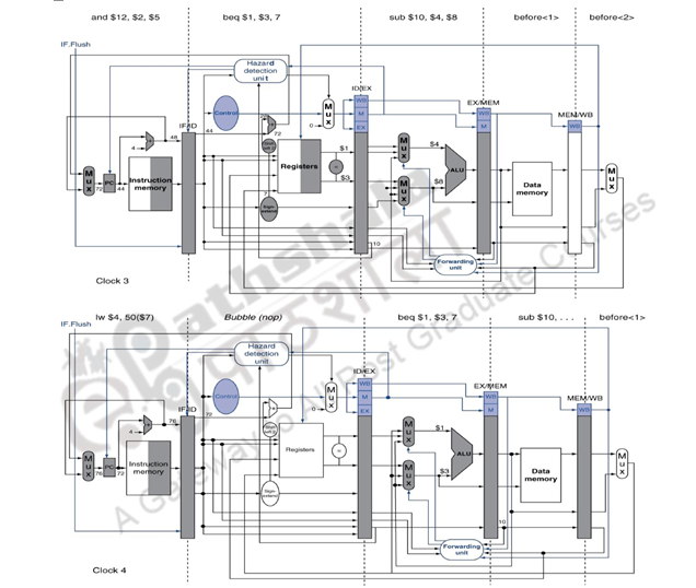
Figure 14.2 shows what happens in the MIPS pipeline when the branch is taken. The ID stage of clock cycle 3 determines that a branch must be taken, so it selects the target address as the next PC address (address 72) and zeros the instruction fetched for the next clock cycle. Clock cycle 4 shows the instruction at location 72 being fetched and the single bubble or nop instruction in the pipeline as a result of the taken branch. The associated data hazards that might arise in the pipeline when the branch is resolved in the second stage has already been discussed in the earlier modules.
Now, we shall discuss the second type of branch prediction, viz. dynamic branch prediction. Branch Prediction is the ability to make an educated guess about which way a branch will go – will the branch be taken or not. In the case of dynamic branch prediction, the hardware measures the actual branch behavior by recording the recent history of each branch, assumes that the future behavior will continue the same way and make predictions. If the prediction goes wrong, the pipeline will stall while re-fetching, and the hardware also updates the history accordingly. The comparison between the static prediction discussed in the earlier module and dynamic prediction is given below:
• Static
– Techniques
• Delayed Branch
• Static prediction
– No info on real-time behavior of programs
– Easier/sufficient for single-issue
– Need h/w support for better prediction
• Dynamic
– Techniques
• History-based Prediction
– Uses info on real-time behavior
– More important for multiple-issue
– Improved accuracy of prediction
In the case of dynamic branch prediction, the hardware can look for clues based on the instructions, or it can use past history. It maintains a History Table that contains information about what a branch did the last time (or last few times) it was executed. The performance of this predictor is
Performance = ƒ(accuracy, cost of mis-prediction)
There are different types of dynamic branch predictors. We shall discuss each of them in detail. The seven schemes that we shall discuss are as follows:
1. 1-bit Branch-Prediction Buffer
2. 2-bit Branch-Prediction Buffer
3. Correlating Branch Prediction Buffer
4. Tournament Branch Predictor
5. Branch Target Buffer
6. Return Address Predictors
7. Integrated Instruction Fetch Units
1-bit Branch-Prediction Buffer: In this case, the Branch History Table (BHT) or Branch Prediction Buffer stores 1-bit values to indicate whether the branch is predicted to be taken / not taken. The lower bits of the PC address index this table of 1-bit values and get the prediction. This says whether the branch was recently taken or not. Based on this, the processor fetches the next instruction from the target address / sequential address. If the prediction is wrong, flush the pipeline and also flip prediction. So, every time a wrong prediction is made, the prediction bit is flipped. Usage of only some of the address bits may give us prediction about a wrong branch. But, the best option is to use only some of the least significant bits of the PC address.
The prediction accuracy of a single bit predictor is not very high. Consider an example of a loop branch taken nine times in a row, and then not taken once. Even in simple iterative loops like this, the 1-bit BHT will cause 2 mispredictions (first and last loop iterations): first time through the loop, when it predicts exit instead of looping, and the end of the loop case, when it exits instead of looping as before. Therefore, the prediction accuracy for this branch that has taken 90% of the time is only 80% (2 incorrect predictions and 8 correct ones). So, we have to look at predictors with higher accuracy.
2-bit predictor: This predictor changes prediction only on two successive mispredictions. Two bits are maintained in the prediction buffer and there are four different states. Two states corresponding to a taken state and two corresponding to not taken state. The state diagram of such a predictor is given below.
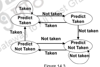
Figure 14.3
Advantage of this approach is that a few atypical branches will not influence the prediction (a better measure of ―the common case‖). Only when we have two successive mispredictions, we will switch prediction. This is especially useful when multiple branches share the same counter (some bits of the branch PC are used to index into the branch predictor). This can be easily extended to N-bits. Suppose we have three bits, then there are 8 possible states and only when there are three successive mispredictions, the prediction will be changed. However, studies have shown that a 2-bit predictor itself is accurate enough.
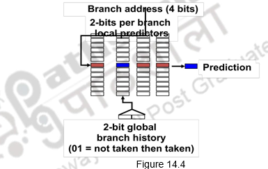
Correlating branch predictors: The 2-bit predictor schemes use only the recent behavior of a single branch to predict the future behavior of that branch. But, many a times, we find that the behavior of one branch is dependent on the behavior of other branches. There is a correlation between different branches. Branch Predictors that use the behavior of other branches to make a prediction are called Correlating or two-level predictors. They make use of global information rather than local behavior information. The information about any number of earlier branches can be maintained. For example, if we maintain the information about three earlier branches, B1, B2 and B3, the behavior of the current branch now depends on how these three earlier branches behaved. There are eight different possibilities, from all three of them not taken (000) to all of them taken (111). There are eight different predictors maintained and each one of them will be maintained as a 1-bit or 2-bit predictor as discussed above. One of these predictors will be chosen based on the behavior of the earlier branches and its prediction used. In general, it is an (m,n) predictor, with global information about m branches and each of the predictors maintained as an n-bit predictor. Figure 14.4 shows an example of a correlating predictor, where m=2.
Tournament predictors: The next type of predictor is a tournament predictor. This uses the concept of ―Predicting the predictor‖ and hopes to select the right predictor for the right branch. There are two different predictors maintained, one based on global information and one based on local information, and the option of the predictor is based on a selection strategy. For example, the local predictor can be used and every time it commits a mistake, the prediction can be changed to the global predictor. Otherwise, the switch can be made only when there are two successive mispredictions. Such predictors are very popular and since 2006, tournament predictors using » 30K bits are used in processors like the Power5 and Pentium 4. They are able to achieve better accuracy at medium sizes (8K – 32K bits) and also make use of very large number of prediction bits very effectively. They are the most popular form of multilevel branch predictors which use several levels of branch-prediction tables together with an algorithm for choosing among the multiple predictors.
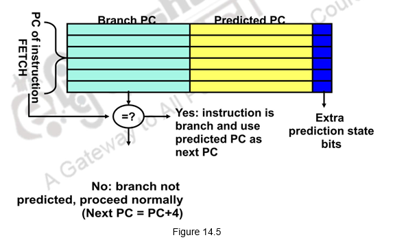
Branch Target Buffer (BTB): With all the branch prediction schemes discussed earlier, we still need to calculate the target address. This gives 1-cycle penalty for a taken branch. If we need to reduce the branch penalty further, we need to fetch an instruction from the destination of a branch quickly. You need the next address at the same time as you’ve made the prediction. This can be tough if you don’t know where that instruction is until the branch has been figured out. The solution is a table that remembers the resulting destination addresses of previous branches. This table is called the Branch Target Buffer (BTB) that caches the target addresses and is indexed by the complete PC value when the instruction is fetched. That is, even before we have decoded the instruction and identified that it is a branch, we index into the BTB. When the PC is used to fetch the next instruction, it is also used to index into the BTB. The BTB stores the PC value and the corresponding target addresses for some of the most recent taken branches. If there is a hit and the instruction is a branch predicted taken, we can fetch the target immediately. This gives a zero cycle penalty for conditional branches. If there is no entry in the BTB, we follow the usual procedure and if it is a taken branch, make an entry in the BTB. On the other hand, if the prediction is wrong, the penalty has to be paid and the BTB entry will have to be removed. This is illustrated in Figure 14.5.
Let us discuss an example problem to illustrate the concepts studied. Consider the table given below.
Determine the total branch penalty for a BTB using the above data. Assume
• Prediction accuracy of 90%
• Hit rate in the buffer of 90% & 60% of the branches are taken
Branch Penalty = Percent buffer hit rate X Percent incorrect predictions X 2 + ( 1 – percent buffer hit rate) X
Taken branches X 2
Branch Penalty = ( 90% X 10% X 2) + (10% X 60% X 2)
Branch Penalty = 0.18 + 0.12 = 0.30 clock cycles
Return Address Predictors: Next we shall at look at the challenge of predicting indirect jumps, that is, jumps whose destination address varies at run time. It is very hard to predict the address for indirect jumps (indirect procedure calls, returns, case statements). If we look at the SPEC89, 85% of such branches are from procedure returns. Though procedure returns can be predicted with a branch-target buffer, the accuracy of such a prediction technique can be low if the procedure is called from multiple sites and the calls from one site are not clustered in time. For example, in SPEC CPU95, an aggressive branch predictor achieves an accuracy of less than 60% for such return branches. To overcome this problem, some designs use a small buffer of return addresses operating as a stack. This structure caches the most recent return addresses: pushing a return address on the stack at a call and popping one off at a return. If the cache is sufficiently large (i.e., as large as the maximum call depth), it will predict the returns perfectly.
Integrated Instruction Fetch Unit: To meet the demands of modern processors that issue multiple instructions every clock cycle, many recent designers have chosen to implement an integrated instruction fetch unit, as a separate autonomous unit that feeds instructions to the rest of the pipeline. An integrated instruction fetch unit integrates several functions:
1. Integrated branch prediction—The branch predictor becomes part of the instruction fetch unit and is constantly predicting branches, so as to drive the fetch pipeline.
2. Instruction prefetch—To deliver multiple instructions per clock, the instruction fetch unit will likely need to fetch ahead. The unit autonomously manages the prefetching of instructions, integrating it with branch prediction.
3. Instruction memory access and buffering—When fetching multiple instructions per cycle a variety of complexities are encountered, including the difficulty that fetching multiple instructions may require accessing multiple cache lines. The instruction fetch unit encapsulates this complexity, using prefetch to try to hide the cost of crossing cache blocks. The instruction fetch unit also provides buffering, essentially acting as an on-demand unit to provide instructions to the issue stage as needed and in the quantity needed.
Thus, as designers try to increase the number of instructions executed per clock, instruction fetch will become an ever more significant bottleneck, and clever new ideas will be needed to deliver instructions at the necessary rate.
To summarize, we have pointed out in this module that prediction is important to handle branch hazards and dynamic branch prediction is more effective. We have discussed different types of predictors. A 1-bit predictor uses one bit prediction, but is not very accurate. A 2-bit predictor has improved prediction accuracies and changes prediction only when there are two successful mispredictions. Correlating branch predictors correlate recently executed branches with the next branch. Tournament Predictors use more resources to competitive solutions and pick between these solutions. A Branch Target Buffer includes the branch address and prediction. Return address stack is used for prediction of indirect jumps. Finally, an integrated instruction fetch unit treats the instruction fetch as a single complicated process and tries to look at different techniques to ensure that a steady stream of instructions are fed to the processor.
Web Links / Supporting Materials
- Computer Organization and Design – The Hardware / Software Interface, David A. Patterson and John L. Hennessy, 4th.Edition, Morgan Kaufmann, Elsevier, 2009.
- Computer Organization, Carl Hamacher, Zvonko Vranesic and Safwat Zaky, 5th.Edition, McGraw- Hill Higher Education, 2011.
Exception handling and floating point pipelines
The objectives of this module are to discuss about exceptions and look at how the MIPS architecture handles them. We shall also discuss other issues that complicate the pipeline.
Exceptions or interrupts are unexpected events that require change in flow of control. Different ISAs use the terms differently. Exceptions generally refer to events that arise within the CPU, for example, undefined opcode, overflow, system call, etc. Interrupts point to requests coming from an external I/O controller or device to the processor. Dealing with these events without sacrificing performance is hard. For the rest of the discussion, we will not distinguish between the two. We shall refer to them collectively as exceptions. Some examples of such exceptions are listed below:
• I/O device request
• Invoking an OS service from a user program
• Tracing instruction execution
• Breakpoint
• Integer arithmetic overflow
• FP arithmetic anomaly
• Page fault
• Misaligned memory access
• Memory protection violation
• Using an undefined or unimplemented instruction
• Hardware malfunctions
• Power failure
There are different characteristics for exceptions. They are as follows:
• Synchronous vs Asynchronous
• Some exceptions may be synchronous, whereas others may be asynchronous. If the same exception occurs in the same place with the same data and memory allocation, then it is a synchronous exception.
They are more difficult to handle.
• Devices external to the CPU and memory cause asynchronous exceptions. They can be handled after the current instruction and hence easier than synchronous exceptions.
• User requested vs Coerced
• Some exceptions may be user requested and not automatic. Such exceptions are predictable and can be handled after the current instruction.
• Coerced exceptions are generally raised by hardware and not under the control of the user program. They are harder to handle.
• User maskable vs unmaskable
• Exceptions can be maskable or unmaskable. They can be masked or unmasked by a user task. This decides whether the hardware responds to the exception or not. You may have instructions that enable or disable exceptions.
• Within vs Between instructions
• Exceptions may have to be handled within the instruction or between instructions. Within exceptions are normally synchronous and are harder since the instruction has to be stopped and restarted. Catastrophic exceptions like hardware malfunction will normally cause termination.
• Exceptions that can be handled between two instructions are easier to handle.
• Resume vs Terminate
• Some exceptions may lead to the program to be continued after the exception and some of them may lead to termination. Things are much more complicated if we have to restart.
• Exceptions that lead to termination are much more easier, since we just have to terminate and need not restore the original status.
Therefore, exceptions that occur within instructions and exceptions that must be restartable are much more difficult to handle.
Exceptions are just another form of control hazard. For example, consider that an overflow occurs on the ADD instruction in the EX stage:
ADD 2, $1
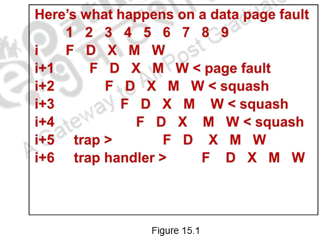
We have to basically prevent $1 from being written into, complete the previous instructions that did not have any problems, flush the ADD and subsequent instructions and handle the exception. This is somewhat similar to a mispredicted branch and we can use much of the same hardware. Normally, once an exception is raised, we force a trap instruction into the pipeline on the next IF and turn off all writes for the faulting instruction and for all instructions that follow in the pipeline, until the trap is taken. This is done by placing zeros in the latches, thus preventing any state changes till the exception is handled. The exception-handling routine saves the PC of the faulting instruction in order to return from the exception later. But if we use delayed branching, it is not possible to re-create the state of the processor with a single PC because the instructions in the pipeline may not be sequentially related. So we need to save and restore as many PCs as the length of the branch delay plus one. This is pictorially depicted in Figure 15.1
Once the exception has been handled, control must be transferred back to the original program in the case of a restartable exception. ISAs support special instructions that return the processor from the exception by reloading the PCs and restarting the instruction stream. For example, MIPS uses the instruction RFE.
If the pipeline can be stopped so that the instructions just before the faulting instruction are completed and those after it can be restarted from scratch, the pipeline is said to have precise exceptions. Generally, the instruction causing a problem is prevented from changing the state. But, for some exceptions, such as floating-point exceptions, the faulting instruction on some processors writes its result before the exception can be handled. In such cases, the hardware must be equipped to retrieve the source operands, even if the destination is identical to one of the source operands. Because floating-point operations may run for many cycles, it is highly likely that some other instruction may have written the source operands. To overcome this, many recent processors have introduced two modes of operation. One mode has precise exceptions and the other (fast or performance mode) does not. The precise exception mode is slower, since it allows less overlap among floating point instructions. In some high-performance CPUs, including Alpha 21064, Power2, and MIPS R8000, the precise mode is often much slower (> 10 times) and thus useful only for debugging of codes.
Having looked at the general issues related to exceptions, let us now look at the
MIPS architecture in particular. The exceptions that can occur in a MIPS pipeline are:
• IF – Page fault, misaligned memory access, memory protection violation
• ID – Undefined or illegal opcode
• EX – Arithmetic exception
• MEM – Page fault on data, misaligned memory access, memory protection violation
• WB – None
In MIPS, exceptions are managed by a System Control Coprocessor (CP0). It saves the PC of the offending or interrupted instruction. A register called the Exception Program Counter (EPC) is used for this purpose. We should also know the cause of the exception. This gives an indication of the problem. MIPS uses a register called the Cause Register to record the cause of the exception. Let us assume two different types of exceptions alone, identified by one bit – undefined instruction = 0 and arithmetic overflow = 1. In order to handle these two registers, we will need to add two control signals EPCWrite and CauseWrite. Additionally, we will need a 1-bit control signal to set the low-order bit of the Cause register appropriately, say, signal IntCause. In the MIPS architecture, the exception handler address is 8000 0180.
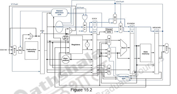
The other way to handle exceptions is by Vectored Interrupts, where the handler address is determined by the cause. In a vectored interrupt, the address to which control is transferred is determined by the cause of the exception. For example, if we consider two different types of exceptions, we can define the two exception vector addresses as Undefined opcode: C0000000, Overflow: C0000020. The operating system knows the reason for the exception by the address at which it is initiated. To summarize, the instructions either deal with the interrupt, or jump to the real handler. This handler reads the cause and transfers control to the relevant handler which determines the action required. If it is a restartable exception, corrective action is taken and the EPC is used to return to the program. Otherwise, the program is terminated and error is reported. Figure 15.2 shows the MIPS pipeline with the EPC and Cause registers added and the exception handler address added to the multiplexor feeding the PC.
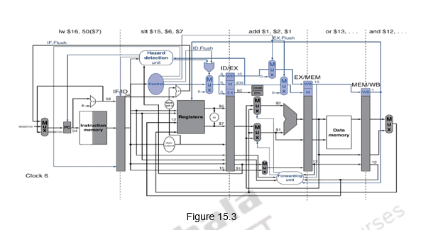
Let us look at an example scenario and discuss what happens in the MIPS pipeline when an exception occurs. Consider the following code snippet and assume that the add instruction raises an exception in the execution stage. This is illustrated in Figure 15.3. During the 6th clock cycle, the add instruction is in the execution stage, the slt instruction is in the decode stage and the lw instruction is in the fetch stage.
40 sub 2, $4
44 and 2, $5
48 or 2, $6
4C add 2, $1
50 slt 6, $7
54 lw 7)
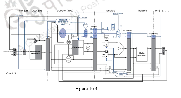
Once the exception in the execution stage is raised, bubbles are inserted in the pipeline starting from the instruction causing a problem, i.e. add in this case. The earlier instructions are allowed to proceed normally. During the next clock cycle, i.e. the 7th clock cycle, a sw 0) instruction is let into the pipeline to handle the exception. This is indicated in Figure 15.4.
Another complication that we need to consider is the fact that multiple exceptions may occur simultaneously, say in the IF and MEM stage and also exceptions may happen out of order. The instruction in the earlier stage, say, IF may raise an exception and then an instruction in the EX stage may raise an exception. Since pipelining overlaps multiple instructions, we could have multiple exceptions at once and also out of order. However, exceptions will have to be handled in order. Normally, the hardware maintains a status vector and posts all exceptions caused by a given instruction in a status vector associated with that instruction. This exception status vector is carried along as the instruction moves down the pipeline. Once an exception indication is set in the exception status vector, any control signal that may cause a data value to be written is turned off (this includes both register writes and memory writes). Because a store can cause an exception during MEM, the hardware must be prepared to prevent the store from completing if it raises an exception. When an instruction enters the WB stage, the exception status vector is checked. If there are any exceptions posted, they are handled in the order in which they would occur in time on an unpipelined processor. Thus, The hardware always deals with the exception from the earliest instruction and if it is a terminating exception, flushes the subsequent instructions. This is how precise exceptions are maintained.
However, in complex pipelines where multiple instructions are issued per cycle, or those that lead to Out-of-order completion because of long latency instructions, maintaining precise exceptions is difficult. In such cases, the pipeline can just be stopped and the status including the cause of the exception is saved. Once the control is transferred to the handler, the handler will determine which instruction(s) had exceptions and whether each instruction is to be completed or flushed. This may require manual completion. This simplifies the hardware, but the handler software becomes more complex.
Apart from the complications caused by exceptions, there are also issues that the ISA can bring in. In the case of the MIPS architecture, all instructions do a write to the register file (except store) and that happens in the last stage only. But is some ISAs, things may be more complicated. For example, when there is support for autoincrement addressing mode, a register write happens in the middle of the instruction. Now, if the instruction is aborted because of an exception, it will leave the processor state altered. Although we know which instruction caused the exception, without additional hardware support the exception will be imprecise because the instruction will be half finished. Restarting the instruction stream after such an imprecise exception is difficult. A similar problem arises from instructions that update memory state during execution, such as the string copy operations on the VAX or IBM 360. If these instructions don’t run to completion and are interrupted in the middle, they leave the state of some of the memory locations altered. To make it possible to interrupt and restart these instructions, these instructions are defined to use the general-purpose registers as working registers. Thus, the state of the partially completed instruction is always in the registers, which are saved on an exception and restored after the exception, allowing the instruction to continue. In the VAX an additional bit of state records when an instruction has started updating the memory state, so that when the pipeline is restarted, the CPU knows whether to restart the instruction from the beginning or from the middle of the instruction. The IA-32 string instructions also use the registers as working storage, so that saving and restoring the registers saves and restores the state of such instructions.
Yet another problem arises because of condition codes. Many processors set the condition codes implicitly as part of the instruction. This approach has advantages, since condition codes decouple the evaluation of the condition from the actual branch.
However, implicitly set condition codes can cause difficulties in scheduling any pipeline delays between setting the condition code and the branch, since most instructions set the condition code and cannot be used in the delay slots between the condition evaluation and the branch. Additionally, in processors with condition codes, the processor must decide when the branch condition is fixed. This involves finding out when the condition code has been set for the last time before the branch. In most processors with implicitly set condition codes, this is done by delaying the branch condition evaluation until all previous instructions have had a chance to set the condition code. In effect, the condition code must be treated as an operand that requires hazard detection for RAW hazards with branches, just as MIPS must do on the registers.
Last of all, we shall look at how the MIPS pipeline can be extended to handle floating point operations. A typical floating point pipeline is shown in Figure 15.5. There are multiple execution units, like FP adder, FP multiply, etc. and they have different latencies. These functional units may or may not be pipelined. We normally define two terms with respect to floating point pipelines. The latency is the number of intervening cycles between an instruction that produces a result and an instruction that uses the result. The initiation or repeat interval is the number of cycles that must elapse between issuing two operations of a given type. The structure of the floating point pipeline requires the introduction of the additional pipeline registers (e.g., A1/A2, A2/A3, A3/A4) and the modification of the connections to those registers. The ID/EX register must be expanded to connect ID to EX, DIV, M1, and A1.
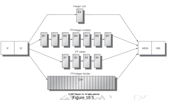
The long latency floating point instructions lead to a more complex pipeline. Since there is more number of instructions in the pipeline, there are frequent RAW hazards. Also, since these floating point instructions have varying latencies, multiple instructions might finish at the same time and there will be potentially multiple writes to the register file in a cycle. This might lead to structural hazards as well as WAW hazards. To handle the multiple writes to the register file, we need to increase the number of ports, or stall one of the writes during ID, or stall one of the writes during WB (the stall will propagate). WAW hazards will have to be detected during ID and the later instruction will have to be stalled. WAR hazards of course, are not possible since all reads happen earlier. The variable latency instructions and hence out-of-order completion will also lead to imprecise exceptions. You either have to buffer the results if they complete early or save more pipeline state so that you can return to exactly the same state that you left at.
To summarize we have discussed the different types of exceptions that might occur in a pipeline and how they can cause problems in the pipeline. We have discussed how the MIPS architecture handles them. Multiple exceptions and out of order exceptions complicate things even more. Certain features of the instruction sets may also complicate the pipeline. Additionally, floating point pipelines have additional complexities to handle.
Web Links / Supporting Materials
- Computer Organization and Design – The Hardware / Software Interface, David A. Patterson and John L. Hennessy, 4th.Edition, Morgan Kaufmann, Elsevier, 2009.
- Computer Organization, Carl Hamacher, Zvonko Vranesic and Safwat Zaky, 5th.Edition, McGraw- Hill Higher Education, 2011.