Advanced Concepts of ILP

Dynamic scheduling

The objectives of this module are to discuss about the advanced concepts used for exploiting ILP and to discuss the concepts of dynamic scheduling in particular.

All processors since about 1985 have used pipelining to overlap the execution of instructions and improve the performance of the processor. This overlap among instructions is called Instruction Level Parallelism since the instructions can be evaluated in parallel. There are two largely separable techniques to exploit ILP:

• Dynamic and depend on the hardware to locate parallelism

• Static and rely much more on software

We know that,

Pipeline CPI = Ideal pipeline CPI + Structural stalls + Data hazard stalls + Control hazard stalls

The ideal pipeline CPI is a measure of the maximum performance attainable by the implementation.

When we look at performing optimizations, and if we only consider the basic block, then, both the compiler as well as the hardware does not have too many options. A basic block is a straight-line code sequence with no branches in, except to the entry, and no branches out, except at the exit. With the average dynamic branch frequency of 15% to 25%, we normally have only 4 to 7 instructions executing between a pair of branches. Additionally, the instructions in the basic block are likely to depend on each other. So, the basic block does not offer too much scope for exploiting ILP. In order to obtain substantial performance enhancements, we must exploit ILP across multiple basic blocks. The simplest method to exploit parallelism is to explore loop-level parallelism, to exploit parallelism among iterations of a loop. Vector architectures are one way of handling loop level parallelism. Otherwise, we will have to look at either dynamic or static methods of exploiting loop level parallelism. One of the common methods is loop unrolling, dynamically via dynamic branch prediction by the hardware, or statically via by the compiler using static branch prediction.

While performing such optimizations, both the hardware as well as the software must preserve program order. That is, the order in which instructions would execute if executed sequentially, one at a time, as determined by the original source program, should be maintained. The data flow, the actual flow of data values among instructions that produce results and those that consume them, should be maintained. Also, instructions involved in a name dependence can execute simultaneously only if the name used in the instructions is changed so that these instructions do not conflict. This is done by the concept of register renaming. This resolves name dependences for registers. This can again be done by the compiler or by hardware. Preserving exception behavior, i.e., any changes in instruction execution order must not change how exceptions are raised in program, should also be considered.

So far, we have assumed static scheduling with in-order-execution and looked at handling all the issues discussed above using various techniques. In this module, we will discuss about the need for doing dynamic scheduling and how we execute instructions out-of-order.

Dynamic Scheduling is a technique in which the hardware rearranges the instruction execution to reduce the stalls, while maintaining data flow and exception behavior. The advantages of dynamic scheduling are:

• It handles cases when dependences are unknown at compile time

– (e.g., because they may involve a memory reference)

• It simplifies the compiler

• It allows code compiled for one pipeline to run efficiently on a different pipeline

• Hardware speculation, a technique with significant performance advantages, builds on dynamic scheduling

In a dynamically scheduled pipeline, all instructions pass through the issue stage in order; however they can be stalled or bypass each other in the second stage and thus enter execution out of order. Instructions will also finish out-of-order.

Score boarding is a dynamic scheduling technique for allowing instructions to execute out of order when there are sufficient resources and no data dependences. But this technique has some drawbacks. The Tomasulo’s algorithm is a more sophisticated technique that has several major enhancements over Score boarding. We will discuss the Tomasulo’s technique here.

The key idea is to allow instructions that have operands available to execute, even if the earlier instructions have not yet executed. For example, consider the following sequence of instructions:

DIV.D F0 , F2 , F4

ADD.D F10 , F0 , F8

SUB.D F12 , F8 , F14

The DIV instruction is a long latency instruction and ADD is dependent on it. So, ADD cannot be executed without DIV finishing. But, SUB has all the operands available, and can be executed earlier than ADD. We are basically enabling out-of-order execution, which will lead to out-of-order completion. With floating point instructions, even with in-order execution, we might have out-of-order completion because of the differing latencies among instructions. Now, with out-of-order execution, we will definitely have out-of-order completion. We should also make sure that no hazards happen in the pipeline because of dynamic scheduling.

In order to allow instructions to execute out-of-order, we need to do some changes to the decode stage. So far, we have assumed that during the decode stage, the MIPS pipeline decodes the instruction and also reads the operands from the register file. Now, with dynamic scheduling, we bring in a change to enable out-of-order execution. The decode stage or the issue stage only decodes the instructions and checks for structural hazards. After that, the instructions will wait until there are no data hazards, and then read operands. This will enable us to do an in order issue, out of order execution and out of order completion. For example, in our earlier example, DIV, ADD and SUB will be issued in-order. But, ADD will stall after issue because of the true data dependency, but SUB will proceed to execution.

There are some disadvantages with dynamic scheduling. They are:

• Substantial increase in hardware complexity

• Complicates exception handling

• Out-of-order execution and out-of-order completion will create the possibility for WAR and WAW hazards. WAR hazards did not occur earlier.

The entire book keeping is done in hardware. The hardware considers a set of instructions called the instruction window and tries to reschedule the execution of these instructions according to the availability of operands. The hardware maintains the status of each instruction and decides when each of the instructions will move from one stage to another. The dynamic scheduler introduces register renaming in hardware and eliminates WAW and WAR hazards. The following example shows how register renaming can be done. There is a name dependence with F6.

• Example:

DIV.DF0,F2,F4

ADD.DF6,F0,F8

S.DF6,0(R1)

SUB.DF8,F10,F14

MUL.D F6,F10,F8

With renaming done as shown below, only RAW hazards remain, which can be strictly ordered.

• Example:

DIV.DF0,F2,F4

ADD.DS,F0,F8

S.DS,0(R1)

SUB.D T,F10,F14

MUL.D F6,F10,T

In the Tomasulo’s approach, the register renaming is provided by reservation stations (RSs). Associated with every functional unit, we have a few reservation stations. When an instruction is issued, a reservation station is allocated to it. The reservation station stores information about the instruction and buffers the operand values (when available). So, the reservation station fetches and buffers an operand as soon as it becomes available (not necessarily involving register file). This helps in avoiding WAR hazards. If an operand is not available, it stores information about the instruction that supplies the operand. The renaming is done through the mapping between the registers and the reservation stations. When a functional unit finishes its operation, the result is broadcast on a result bus, called the common data bus (CDB). This value is written to the appropriate register and also the reservation station waiting for that data. When two instructions are to modify the same register, only the last output updates the register file, thus handling WAW hazards. Thus, the register specifiers are renamed with the reservation stations, which may be more than the registers. For load and store operations, we use load and store buffers, which contain data and addresses, and act like reservation stations.

The three steps in a dynamic scheduler are listed below:

• Issue

• Get next instruction from FIFO queue

• If available RS, issue the instruction to the RS with operand values if available

• If a RS is not available, it becomes a structural hazard and the instruction stalls

• If an earlier instruction is not issued, then subsequent instructions cannot be issued

• If operand values not available, stall the instruction

• Execute

• When operand becomes available, store it in any reservation station waiting for it

• When all operands are ready, issue the instruction for execution

• Loads and store are maintained in program order through the effective address

• No instruction allowed to initiate execution until all branches that proceed it in program order have completed

• Write result

• Write result on CDB into reservation stations and store buffers

• Stores must wait until address and value are received

The dynamic scheduler maintains three data structures – the reservation station, a register result data structure that keeps of the instruction that will modify a register and an instruction status data structure. The third one is more for understanding purposes. The reservation station components are as shown below:

Name —Identifying the reservation station

Op—Operation to perform in the unit (e.g., + or –)

Vj, Vk—Value of Source operands

– Store buffers have V field, result to be stored

Qj, Qk—Reservation stations producing source registers (value to be written)

– Store buffers only have Qi for RS producing result Busy—Indicates reservation station or FU is busy

Register result status—Indicates which functional unit will write each register, if one exists. It is blank when there are no pending instructions that will write that register. The instruction status gives the status of each instruction in the instruction window. All the three data structures are shown in Figure 16.1.

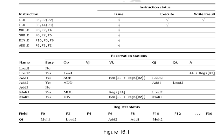
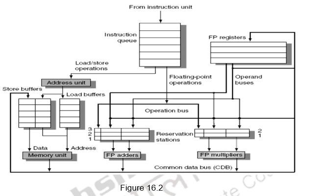
Figure 16.2 shows the organization of the Tomasulo’s dynamic scheduler. Instructions are taken from the instruction queue and issued. During the issue stage, the instruction is decoded and allocated an RS entry. The RS station also buffers the operands if available. Otherwise, the RS entry marks the pending RS value in the Q field. The results are passed through the CDB and go to the appropriate register, as dictated by the register result data structure, as well as the pending RSs.

Dependences with respect to memory locations will also have to be handled properly. A load and a store can safely be done out of order, provided they access different addresses. If a load and a store access the same address, then either

the load is before the store in program order and interchanging them results in a WAR hazard, or
the store is before the load in program order and interchanging them results in a RAW hazard.

Similarly, interchanging two stores to the same address results in a WAW hazard. Hence, to determine if a load can be executed at a given time, the processor can check whether any uncompleted store that precedes the load in program order shares the same data memory address as the load. Similarly, a store must wait until there are no unexecuted loads or stores that are earlier in program order and share the same data memory address.

To summarize, we have discussed the importance of dynamic scheduling, wherein the hardware does a dynamic reorganization of code at run time. We have discussed the Tomasulo’s dynamic scheduling approach. The book keeping done and the various steps used have been elaborated.

Web Links / Supporting Materials

Computer Organization and Design – The Hardware / Software Interface, David A. Patterson and John L. Hennessy, 4th Edition, Morgan Kaufmann, Elsevier, 2009.
Computer Architecture – A Quantitative Approach , John L. Hennessy and David A. Patterson, 5th Edition, Morgan Kaufmann, Elsevier, 2011.

Dynamic scheduling – Example

The objective of this module is to go through a clock level simulation for a sequence of instructions that undergo dynamic scheduling. We will look at how the data structures maintain the relevant information and how the hazards are handled.

We will first of all do a recap of dynamic scheduling. Dynamic Scheduling is a technique in which the hardware rearranges the instruction execution to reduce the stalls, while maintaining data flow and exception behavior. The advantages of dynamic scheduling are:

• It handles cases when dependences are unknown at compile time

– (e.g., because they may involve a memory reference)

• It simplifies the compiler

• It allows code compiled for one pipeline to run efficiently on a different pipeline

• Hardware speculation, a technique with significant performance advantages, builds on dynamic scheduling

The three steps in a dynamic scheduler are listed below

• Issue

• Get next instruction from FIFO queue

• If available RS, issue the instruction to the RS with operand values if available

• If a RS is not available, it becomes a structural hazard and the instruction stalls

• If an earlier instruction is not issued, then subsequent instructions cannot be issued

• If operand values are not available, the instructions will wait in the RSs looking at CDBs for operands

• Execute

• When operand becomes available on the CDB, store it in any reservation station waiting for it

• When all operands are ready, the instruction is executed by the respective functional unit

• Loads and store are maintained in program order through the effective address

• No instruction allowed to initiate execution until all branches that proceed it in program order have completed

• Write result

• Write result on CDB into reservation stations and store buffers

• Stores must wait until address and value are received

Name —Identifying the reservation station

Op—Operation to perform in the unit (e.g., + or –)

Vj, Vk—Value of Source operands

– Store buffers have V field, result to be stored

Qj, Qk—Reservation stations producing source registers (value to be written)

– Store buffers only have Qi for RS producing result

Busy—Indicates reservation station or FU is busy

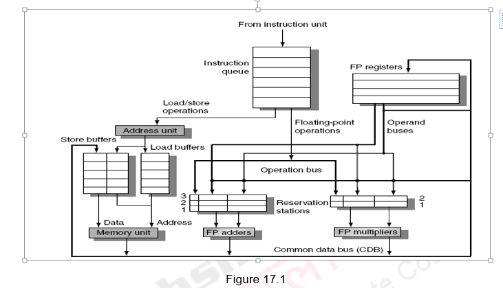
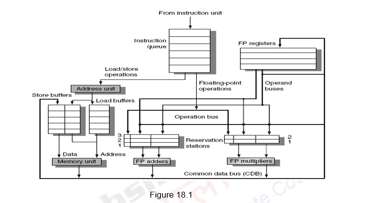
Figure 17.1 shows the organization of the Tomasulo’s dynamic scheduler. Instructions are taken from the instruction queue and issued. During the issue stage, the instruction is decoded and allocated an RS entry. The RS station also buffers the operands if available. Otherwise, the RS entry marks the pending RS value in the Q field. The results are passed through the CDB and go to the appropriate register, as dictated by the register result data structure, as well as the pending RSs.

Having looked at the basics of the Tomasulo’s dynamic scheduler, we shall now discuss how dynamic scheduling happens for a sequence of instructions. We are only considering a basic block without branches.

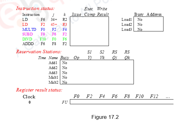
Figure 17.2 shows the sequence of instructions considered along with the three data structures maintained. We shall assume three Add reservation stations and two Mul reservation stations. There are also three Load buffers. Assume that Add has a latency of 2, Mul has a latency of 10 and Div has a latency of 40.

During the first clock cycle, Load1 is issued. A load buffer entry is allocated, its status is now busy and the contents of R2 needed for the effective address calculation and the value 34 is stored in the buffer. The register result status shows that register F6 is to be written by the instruction identified by Load buffer1.

During the second clock cycle, Load1 moves from the issue stage to the execution stage. The effective address (34+R2) is calculated and stored in the Load buffer1. Meanwhile, instruction 2, i.e. Load2 is issued. It is allocated Load buffer entry2, and the details of the effective address (45, R3) are stored there. Load buffer2 is now busy. The register result status shows that register F2 is to be written by the instruction identified by Load buffer2.

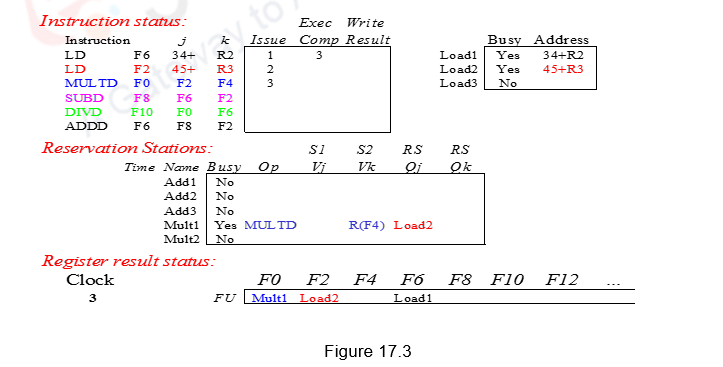
During the third clock cycle, Load1 does the memory access and completes execution. For Load2, the effective address (45+R3) is calculated and stored in the Load buffer2. Meanwhile, instruction 3, i.e. Mul is issued. It is allocated Mult1 entry, the contents of register F4 are fetched and stored in the place of V_k. The other operand F2 cannot be fetched now and has to wait for Load2 to finish. This is indicated in the Q_j field as Load2. Mult1 reservation station is marked busy. The register result status shows that register F0 is to be written by the instruction identified by Mult1. This scenario is indicated in Figure 17.3.

During the fourth clock cycle, Load1 writes the result on the CDB and the corresponding Load1 entry is made free. This data on the CDB writes into F6. Load2 does the memory access and completes execution. Meanwhile, instruction 4, i.e. Sub is issued. It is allocated Add1 entry, the contents of register F6 are fetched and stored in V_j. The other operand F2 cannot be fetched now and has to wait for Load2 to finish. This is indicated in the Q_k field as Load2. Add1 reservation station is marked busy. The register result status shows that register F8 is to be written by the instruction identified by Add1. Note that Mul is still waiting for the operand and is stalled.

During the fifth clock cycle, Load2 writes the result on the CDB and the corresponding Load2 entry is made free. This data on the CDB writes into F2. This data is taken up by the Mult1 reservation station and the Add1 reservation station that have been waiting. These two instructions, Sub and Mul are now ready for execution. Meanwhile, instruction 5, i.e. Div is issued. It is allocated Mult2 entry, the contents of register F6 are fetched and stored in V_k. The other operand F0 cannot be fetched now and has to wait for Mul to finish. This is indicated in the Q_j field as Mult1. Mult2 reservation station is marked busy. The register result status shows that register F10 is to be written by the instruction identified by Mult2 (Div instruction).

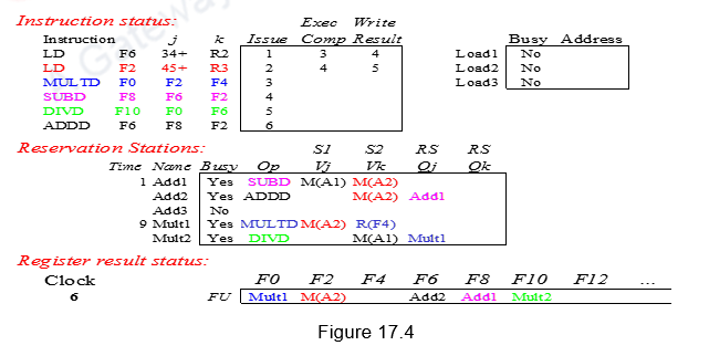
During the sixth clock cycle, both the Mul instruction and the Sub instruction have gone through one execution cycle. Meanwhile, instruction 6, i.e. Add is issued. It is allocated Add2 entry, the contents of register F2 are fetched and stored in V_k. The other operand F8 cannot be fetched now and has to wait for Sub to finish. This is indicated in the Q_j field as Add1. Add2 reservation station is marked busy. The register result status shows that register F6 is to be written by the instruction identified by Add2 (Add instruction). This scenario is depicted in Figure 17.4.

Note that there is a name dependency for F6 for the Add instruction with both the Div as well as the Sub instruction, which might lead to WAR hazards. However, since the operand F6 for both the Sub and Div instructions have already been read and buffered in the respective reservation stations, the name dependency has been resolved by register renaming and thus avoids the possible WAR hazards.

The Sub instruction finishes execution in the seventh clock cycle, since it has a latency of 2. Nothing else happens in this clock cycle. It writes into the CDB in the eighth clock cycle. The result of Sub is written into the register F8 and it also writes into the reservation station Add2 of the Add subtraction. The Add1 entry is now freed up.

Clock cycle nine – Add and Mul are still executing. During clock cycle ten, Add finishes execution and it writes into the CDB in clock cycle eleven. This data goes into register F6 and the Add2 reservation station entry is freed up. Note that even though there is a name dependency on register F6 with the Div instruction, this does not cause a problem. The Div instruction‘s reservation station has already got the original data of F6 through the Load1 instruction.

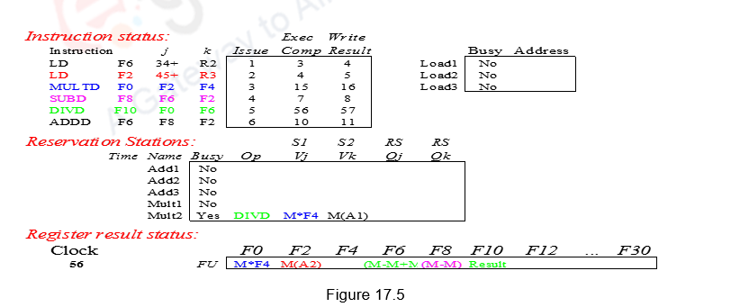
During clock cycle fifteen, Mul finishes execution (latency of 10 – clock cycle six to fifteen) and it writes the result in clock cycle sixteen. The result goes to register F0 and the reservation station Mult2 waiting for it (Div instruction). The Mult1 entry is freed up. Div starts executing in clock cycle seventeen and finishes execution in fifty six (latency of 40). It writes the result in fifty seven and frees up the Mult2 entry. The complete schedule is shown in Figure 17.5. Observe the instructions are issued in-order, execute out-of-order and complete execution out-of-order.

The advantages of the Tomasulo’s dynamic scheduling approach are as follows:

(1) The distribution of the hazard detection logic:

– Tomasulo’s approach uses distributed reservation stations and the CDB

– If multiple instructions are waiting on a single result, and each instruction has other operand, then instructions can be released simultaneously by broadcast on CDB

– If a centralized register file were used, the units would have to read their results from the registers when register buses are available.

(2) The elimination of stalls for WAW and WAR hazards

– The buffering of the operands in the reservation stations, as soon as they become available, does the mapping between the registers and the reservation stations. This renaming process avoids WAR hazards. Even if a subsequent instruction modifies the register file, there is no problem because the operand has already been read and buffered.

– When two or more instructions write into the same register, leading to WAW hazards, only the latest register information is maintained in the register result status. This renaming avoids WAW hazards.

However, this approach is not without drawbacks. The following are the drawbacks:

· Complexity

o The hardware becomes complicated with the book keeping done and the CDB and the associative compares

· Many associative stores (CDB) at high speed

· Performance limited by Common Data Bus

o Each CDB must go to multiple functional units. This leads to high capacitance and high wiring density

o With only one CDB, the number of functional units that can complete per cycle is limited to one!

§ Multiple CDBs will lead to more FU logic for parallel associative stores

· Non-precise interrupts!

o The out-of-order execution will lead to non-precise interrupts. We will address this later when we discuss speculation.

We have not discussed dependences with respect to memory locations. They will also have to be handled properly. A load and a store can safely be done out of order, provided they access different addresses. If a load and a store access the same address, then either

· the load is before the store in program order and interchanging them results in a WAR hazard, or

· the store is before the load in program order and interchanging them results in a RAW hazard.

To summarize, we have discussed an example of dynamic scheduling, wherein the hardware does a dynamic reorganization of code at run time. For a given sequence of instructions, we have looked at a clock level simulation. The book keeping done and the various steps used have been elaborated. We have not handled branches in this example.

Web Links / Supporting Materials

Computer Organization and Design – The Hardware / Software Interface, David A. Patterson and John L. Hennessy, 4th Edition, Morgan Kaufmann, Elsevier, 2009.

Computer Architecture – A Quantitative Approach , John L. Hennessy and David A. Patterson, 5th Edition, Morgan Kaufmann, Elsevier, 2011.

Dynamic scheduling – Loop Based Example

The objective of this module is to go through a clock level simulation for a sequence of instructions including branches that undergo dynamic scheduling. We will look at how the data structures maintain the relevant information and how the hazards are handled.

It handles cases when dependences are unknown at compile time
- – (e.g., because they may involve a memory reference)
It simplifies the compiler
It allows code compiled for one pipeline to run efficiently on a different pipeline
Hardware speculation, a technique with significant performance advantages, builds on dynamic scheduling

In order to allow instructions to execute out-of-order, we need to do some changes to the decode stage. So far, we have assumed that during the decode stage, the MIPS pipeline decodes the instruction and also reads the operands from the register file. Now, with dynamic scheduling, we bring in a change to enable out-of-order execution. The decode stage or the issue stage only decodes the instructions and checks for structural hazards. If there is no structural hazard, i.e. a reservation station available, the instruction is issued. After that, the instructions will wait in the reservation stations until the dependent instructions produce data, and then read operands. This will enable us to do an in order issue, out of order execution and out of order completion.

The three steps in a dynamic scheduler are listed below:

Issue
- Get next instruction from FIFO queue
- If available RS, issue the instruction to the RS with operand values if available
- If a RS is not available, it becomes a structural hazard and the instruction stalls
- If an earlier instruction is not issued, then subsequent instructions cannot be issued
- If operand values are not available, the instructions wait for the operands to arrive on the CDBs
Execute
- When operand becomes available, store it in any reservation station waiting for it
- When all operands are ready, issue the instruction for execution
- Loads and store are maintained in program order through the effective address
- No instruction allowed to initiate execution until all branches that proceed it in program order have completed
Write result
- Write result on CDB into reservation stations and store buffers
  - Stores must wait until address and value are received

The dynamic scheduler maintains three data structures – the reservation station, a register result data structure that keeps track of the instruction that will modify a register and an instruction status data structure. The third one is more for understanding purposes. The reservation station components are as shown below:

Name —Identifying the reservation station

Op—Operation to perform in the unit (e.g., + or –)

Vj, Vk—Value of Source operands

– Store buffers have V field, result to be stored

Qj, Qk—Reservation stations producing source registers (value to be written)

– Store buffers only have Qi for RS producing result

Busy—Indicates reservation station or FU is busy

Figure 18.1 shows the organization of the Tomasulo’s dynamic scheduler. Instructions are taken from the instruction queue and issued. During the issue stage, the instruction is decoded and allocated an RS entry. The RS station also buffers the operands if available. Otherwise, the RS entry marks the pending RS value in the Q field. The results are passed through the CDB and go to the appropriate register, as dictated by the register result data structure, as well as the pending RSs.

Having looked at the basics of the Tomasulo’s dynamic scheduler, we shall now discuss how dynamic scheduling happens for a sequence of instructions. The previous module discussed a case where there were no branches. When we look at performing optimizations, and if we only consider the basic block, then, both the compiler as well as the hardware does not have too many options. A basic block is a straight-line code sequence with no branches in, except to the entry, and no branches out, except at the exit. With the average dynamic branch frequency of 15% to 25%, we normally have only 4 to 7 instructions executing between a pair of branches. Additionally, the instructions in the basic block are likely to depend on each other. So, the basic block does not offer too much scope for exploiting ILP. In order to obtain substantial performance enhancements, we must exploit ILP across multiple basic blocks. The simplest method to exploit parallelism is to explore loop-level parallelism, to exploit parallelism among iterations of a loop. Vector architectures are one way of handling loop level parallelism. Otherwise, we will have to look at either dynamic or static methods of exploiting loop level parallelism. One of the common methods is loop unrolling, dynamically via dynamic branch prediction by the hardware, or statically via by the compiler using static branch prediction.

This example with loops will illustrate how the hardware dynamically unrolls the loop using dynamic branch prediction. We also assume that instructions beyond the branch are fetched and issued based on the dynamic branch predictor’s prediction. However, these instructions beyond the branch are not executed till the branch is resolved. This is because of the fact that, if the branch prediction fails and we have already executed instructions and written into memory or the register file, it cannot be undone. That is, we are not speculatively executing instructions.

Let us consider the loop as shown below.

Loop: LD F0 0 R1

MULTD F4 F0 F2

SD F4 0 R1

SUBI R1 R1 #8

BNEZ R1 Loop

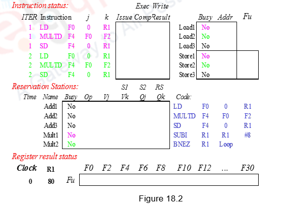
Figure 18.2 shows the sequence of instructions considered along with the three data structures maintained. We shall assume three Add reservation stations and two Mul reservation stations. There are also three load buffers and three store buffers. Assume that Add has a latency of 2, Multiply takes 4 clocks, the first load takes 8 clocks because of a L1 cache miss and the second load takes 1 clock (hit). We shall consider two iterations of the loop. R1 register is initialized to 80, so that the loop gets executed 10 times. For the simulation to be clear, we will show clocks for the integer instructions SUBI and BNEZ. However, in reality, these integer instructions will be ahead of the floating point Instructions.

During the first clock cycle, Load1 is issued. A load buffer entry is allocated, its status is now busy and the contents of R1 needed for the effective address calculation and the value 0 is stored in the buffer. The register result status shows that register F0 is to be written by the instruction identified by Load buffer1.

During the second clock cycle, Load1 moves from the issue stage to the execution stage. The effective address (0+R1) is calculated (80) and stored in the Load buffer1. Meanwhile, instruction 2, i.e. Mul1 is issued. It is allocated Mult1 entry, the contents of register F2 are fetched and stored in the place of Vk. The other operand F0 cannot be fetched now and has to wait for Load1 to finish. This is indicated in the Qj field as Mult1. Mult1 reservation station is marked busy. The register result status shows that register F4 is to be written by the instruction identified by Mult1.

During the third clock cycle, Store1 is issued. The store buffer entry Store1 is allocated for this store. The values 0 and (R1) for the effective address calculation are stored there. Also, the data field indicates that Mult1 has to produce the data for Store1. Note that Load1 has a cache miss and has not performed the memory access. The Mul1 instruction needs data from the Load1 instruction and is also stalled. This scenario is indicated in Figure 18.3.

During the fourth clock cycle, the Sub instruction is issued to the integer unit. Store calculates the effective address (80) and stores in the Store1 entry. During the fifth clock cycle, the Branch instruction is issued to the integer unit.

During the sixth clock cycle, assuming that the branch predictor predicts the branch to be taken, dynamic unrolling of the loop is done and Load2 of the second iteration is issued to Load2 entry. This entry is marked busy. The register result status shows that register F0 is to be written by the instruction identified by Load2. Note that though we are using the same register F0 for both the load instructions, a WAW hazard does not happen because the later of the two loads is only writing into F0. Meanwhile, the Sub instruction finishes completion.

During the seventh clock cycle, the Mul instruction of the second iteration is issued. It is allocated Mult2 entry, the contents of register F2 are fetched and stored in Vk. The other operand F0 cannot be fetched now and has to wait for Load2 to finish. This is indicated in the Qj field as Load2. Mult2 reservation station is marked busy. The register result status shows that register F4 is to be written by the instruction identified by Mult2. This overwrites the fact that F4 has to modify register F4, avoiding WAW hazard. Observe that the renaming allows the register file to be completely detached from the computation and the first and second iterations are completely overlapped. The Sub instruction writes its result. The Branch is data dependent on Sub and has not yet executed. Because of this, the Load2 after Branch does not do execution.

During the eighth clock cycle, Store2 is issued. The store buffer entry Store2 is allocated for this store. Also, the data field indicates that Mult2 has to produce the data for Store2. Note that Load1 has not yet finished the memory access. The Mul instructions need data from the Load instructions and are also stalled. The Branch instruction is resolved in this clock cycle.

During the ninth clock cycle, the effective address calculation for Load2 and Store2 happens. Meanwhile, Load1 finishes execution (latency 7 – clock cycles 3-9) and the Sub of the second iteration is issued. The tenth clock cycle does the write of the Load1 result on the CDB also filling the Mult1 data. The second Branch instruction is also issued. The Load2 instruction also does a memory access here.

During the eleventh clock cycle, Mul1 starts executing and the Load2 writes the result on the CDB and hence the register F0. Sub2 finishes execution. Note that the initial loaded value from Load1 is never written into F0. Load2 has produced the data for Mult2 and so the Mul2 instruction is now ready for execution. Load3 is issued in this clock cycle.

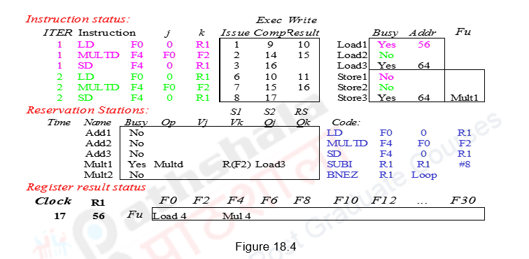
During the twelfth clock cycle, Mul2 starts executing and Sub2 writes its result. The third Mul instruction cannot be issued as there is a structural hazard (no Mult reservation station). The second Branch gets resolved in clock cycle thirteen. The Mul1 instruction finishes in clock cycle fourteen and the Mul2 instruction finishes execution in clock cycle fifteen. Mul1 writes the result in fifteen and Mul2 writes the result in sixteen. Therefore, Store1 completes in sixteen and Store2 completes in seventeen. Only in the sixteenth clock cycle, Mul3 can be issued and the other instructions can be issued in subsequent clock cycles. The final schedule is shown in Figure 18.4.

Observe that there is an in-order issue, out-of-order execution and out-of-order completion. Due to the renaming process, multiple iterations use different physical destinations for the registers (dynamic loop unrolling). This is why the Tomasulo’s approach is able to overlap multiple iterations of the loop. The reservation stations permit instruction issue to advance past the integer control flow operations. They buffer the old values of registers, thus totally avoiding the WAR stall that would have happened otherwise. Thus we can say that the Tomasulo’s approach builds the data flow dependency graph on the fly. However, the performance improvement depends on the accuracy of the branch prediction. If the branch prediction goes wrong, the instructions fetched and issued from the wrong path will have to be discarded, leading to penalty.

The advantages of the Tomasulo’s dynamic scheduling approach are as follows:

(1) The distribution of the hazard detection logic:
- – Tomasulo’s approach uses distributed reservation stations and the CDB
- – If multiple instructions are waiting on a single result, and each instruction has other operand, then instructions can be released simultaneously by broadcast on CDB
- – If a centralized register file were used, the units would have to read their results from the registers when register buses are available.
(2) The elimination of stalls for WAW and WAR hazards
- – The buffering of the operands in the reservation stations, as soon as they become available, does the mapping between the registers and the reservation stations. This renaming process avoids WAR hazards. Even if a subsequent instruction modifies the register file, there is no problem because the operand has already been read and buffered.
- – When two or more instructions write into the same register, leading to WAW hazards, only the latest register information is maintained in the register result status. This renaming avoids WAW hazards.

However, this approach is not without drawbacks. The following are the drawbacks:

Complexity
- o The hardware becomes complicated with the book keeping done and the CDB and the associative compares
Many associative stores (CDB) at high speed
Performance limited by Common Data Bus
- o Each CDB must go to multiple functional units. This leads to high capacitance and high wiring density
- o With only one CDB, the number of functional units that can complete per cycle is limited to one!
  - Multiple CDBs will lead to more FU logic for parallel associative stores
- Non-precise interrupts!
  - o The out-of-order execution will lead to non-precise interrupts. We will address this later when we discuss speculation.

the load is before the store in program order and interchanging them results in a WAR hazard, or
the store is before the load in program order and interchanging them results in a RAW hazard.

Similarly, interchanging two stores to the same address, results in a WAW hazard. Hence, to determine if a load can be executed at a given time, the processor can check whether any uncompleted store that precedes the load in program order shares the same data memory address as the load. Similarly, a store must wait until there are no unexecuted loads or stores that are earlier in program order and share the same data memory address.

To summarize, we have looked at an example for dynamic scheduling with branches, wherein the hardware does a dynamic reorganization of code at run time. Based on the branch prediction, branches are dynamically unrolled. Instructions beyond the branch are fetched and issued, but not executed. The book keeping done and the various steps carried out during every clock cycle have been elaborated.

Web Links / Supporting Materials

Computer Organization and Design – The Hardware / Software Interface, David A. Patterson and John L. Hennessy, 4th Edition, Morgan Kaufmann, Elsevier, 2009.

Computer Architecture – A Quantitative Approach , John L. Hennessy and David A. Patterson, 5th Edition, Morgan Kaufmann, Elsevier, 2011.

Dynamic scheduling with Speculation

The objective of this module is to go through the concept of hardware speculation and discuss how dynamic scheduling can be enhanced with speculation. We will look at how the data structures maintain the relevant information and how the hazards are handled.

It handles cases when dependences are unknown at compile time
- – (e.g., because they may involve a memory reference)
It simplifies the compiler
It allows code compiled for one pipeline to run efficiently on a different pipeline
Hardware speculation, a technique with significant performance advantages, builds on dynamic scheduling

The dynamic scheduling technique that we discussed in the previous modules did not allow the processor to execute instructions beyond a branch. The dynamic branch prediction facilitates dynamic unrolling of loops. However, instructions after the branch can only be fetched and decoded, they cannot be executed. This is because of the fact that there is no provision to undo the effects of the instruction, if the branch prediction fails. But, that again limits the parallelism that can be exploited. So, if we need to uncover more parallelism, we need to execute instructions even before the branch is resolved. This concept of speculatively executing instructions before the branch is resolved, is called hardware speculation. During every cycle, the processor executes an instruction – even if it may be the wrong instruction. This is yet another way of overcoming control dependence – by speculating on the outcome of branches and executing the program as if our guesses were correct. Obviously, if our guesses go wrong, we should have the provision to undo. We are essentially building a data flow execution model, so as to execute instructions as soon as the operands are available. The details of this speculative execution are discussed in this module.

There are three components to dynamic scheduling with speculation. They are:

Dynamic branch prediction to choose which instructions to execute
Speculation to allow the execution of instructions before the control dependence is resolved
- o Support to undo if prediction is wrong
Dynamic scheduling to deal with the scheduling of different combinations of basic blocks Processors like the PowerPC 603/604/G3/G4, MIPS R10000/R12000, Intel Pentium II/III/4, i3, i5, i7, Alpha 21264, AMD K5/K6/Athlon, etc. use dynamic scheduling with speculation.

Hardware Based Speculation: Earlier, with dynamic scheduling, instructions after the branch were executed only after the branch was resolved. So, during the write back stage, they wrote into registers or memory. Now, with speculation, we execute instructions along predicted execution paths, and the results can only be committed if the prediction was correct. Instruction commit allows an instruction to update the register file or memory only when the instruction is no longer speculative.

This indicates that we need an additional piece of hardware that will buffer the results of the instruction till they commit. This piece of hardware is called the Reorder Buffer, abbreviated as ROB. This helps to prevent any irrevocable action until an instruction commits, i.e. updating state or taking an execution. The reorder buffer holds the result of an instruction from the time it executes to the time it commits. It is also used to pass operands among speculated instructions.

The reorder buffer has the following fields. They are:

Name or tag field for identification
Instruction type: branch/store/register
Destination field : register number
Value field: output value
Ready field: completed execution?

The ROB extends the architectural registers just like the reservation stations. With support for speculation, we now identify an instruction using its ROB entry and not the reservation station entry. The reservation station holds the operands from the time an instruction is issued to the time it executes. The ROB buffers the result from the time an instruction executes to the time it commits. However, we are looking at an in-order commit and an ROB entry is assigned when the instruction is issued itself. The mapping is done between the registers, the reservation stations and the ROB. This helps avoiding WAW and WAR hazards. To handle control hazards, the speculated entries in the ROB are cleared if there is a misprediction, Just note that exceptions are not recognized until the instruction causing exception is ready to commit. We shall discuss more about this later on.

The overall architecture of a dynamic scheduler with speculation is given in Figure 19.1. It is the same as the architecture that we discussed in the earlier modules, with the addition of an ROB.

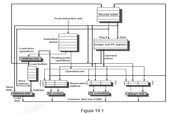
Instructions are taken from the prefetched instruction queue and decoded. The decode stage or the issue stage decodes the instructions and checks for structural hazards. The unavailability of a reservation station or an ROB entry leads to a structural hazard. A reservation station entry is allocated depending on the type of instruction, whereas an ROB entry is allocated sequentially (in-order issue and in-order commit). Since we are looking at an in-order issue, if an instruction stalls at the issue stage, the subsequent instructions cannot be issued. After that, the instructions will wait until there are no data hazards, and then read operands. This will enable us to do an in order issue, out of order execution and out of order completion. After the results are computed, the results are written only into the appropriate ROB entry and the reservation stations waiting for this data. Note that the CDB writes only into the ROB and the reservation stations, and not the register file. Another change is that we do not have separate store buffers. The ROB entries themselves act as store buffer entries. They buffer the store address and the data to be stored till the store instructions’ turn for commit arrives. The register result status indicates which register is to be written by which ROB tag. During the commit stage, data is either transferred from the ROB to registers or memory. If the committed instruction is a branch, the prediction is checked and if the prediction was correct, the branch is removed from the ROB queue and the subsequent instructions are committed in-order. Otherwise, the branch is removed and the ROB is flushed.

The entire book keeping is done in hardware. The hardware considers a set of instructions called the instruction window and tries to reschedule the execution of these instructions according to the availability of operands. The hardware maintains the status of each instruction and decides when each of the instructions will move from one stage to another. Register renaming is done in hardware with the help of the reservation stations and the ROB. This eliminates WAW and WAR hazards.

Apart from the three steps in the dynamic scheduler, an additional step of commit is introduced when there is support for speculation. The four steps in a dynamic scheduler with speculation are listed below:

Issue
- Get next instruction from FIFO queue
- If available RS entry and ROB entry, issue the instruction
- If a RS or ROB entry is not available, it becomes a structural hazard and the instruction stalls
- If an earlier instruction is not issued, then subsequent instructions cannot be issued
- If operands are available read them and store them in the reservation station
  - Operands can be read from the register file (already committed instructions) or from the ROB (executed but not yet committed)
- Operands dependent on an earlier instruction are identified by their corresponding ROB tag in the Q field and such instructions will have to stall till data becomes available
Execute
- The CDB broadcasts data with an ROB tag and when an operand becomes available, store it in any reservation station waiting for it
- When all operands are ready, issue the instruction for execution
- Free the reservation station entry once the instruction moves into execution
- Loads and store are maintained in program order through the effective address
- Even with pending branches, instructions are speculatively executed
Write result
- Write result on CDB into reservation stations and ROB
Commit
- An instruction is committed when it reaches the head of the ROB and its result is present in the buffer
- If it is an ALU or Load instruction, update the register with the result and remove the instruction from the ROB
- Committing a store is similar except that memory is updated rather than a result register
- If a branch with incorrect prediction reaches the head of the ROB, it indicates that the speculation was wrong
  - ROB is ﬂushed and execution is restarted at the correct successor of the branch
- If the branch was correctly predicted, the branch is removed from ROB
- Once an instruction commits, its entry in the ROB is reclaimed.
- If the ROB ﬁlls, we simply stop issuing instructions until an entry is made free.

The dynamic scheduler with speculation maintains four data structures – the reservation station, ROB, a register result data structure that keeps track of the ROB entry that will modify a register and an instruction status data structure. The last one is more for understanding purposes.

Having looked at the basics of a dynamic scheduler with speculation, we shall now discuss how the scheduling happens for a sequence of instructions. Let us consider the sequence of instructions that we discussed earlier for dynamic scheduling. Assume the latencies for the Add, Mul and Div instructions to be 2, 6 and 12 respectively.

L.D F6,32(R2)

L.D F2,44(R3)

MUL.D F0,F2,F4

SUB.D F8,F6,F2

DIV.D F10,F0,F6

ADD.D F6,F8,F2

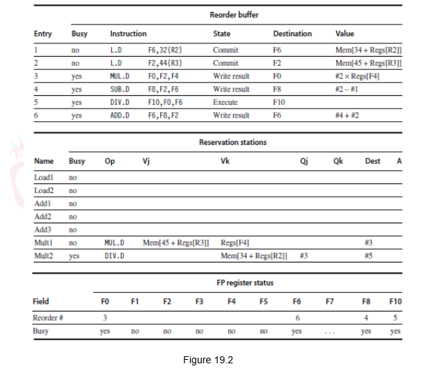
Figure 19.2 shows how the status tables will look like when the MUL.D is ready to go to commit. Observe that though the Sub and Add instructions have written the result, they have not yet committed. This is because the Mul instruction has not yet committed. The Dest field designates the ROB entry that is the destination for the result produced by a particular reservation station entry. The complete schedule is given in Table 19.1.

Instruction	Issues at	Executes at	Writes result at	Commits at
L.D F6,32(R2)	1	2-3	4	5
L.DF2,44(R3)	2	3-4	5	6
MUL.D F0,F2,F4	3	6-11	12	13
SUB.D F8,F6,F2	4	6-7	8	14
DIV.D F10,F0,F6	5	13-24	25	26
ADD.D F6,F8,F2	6	9-10	11	27

Table 19.1

Note that the instructions are issued in-order, executed out-of-order, completed out-of-order, but committed in-order.

One implication of speculative execution is that it maintains a precise exception model. For example, if the MUL.D instruction caused an exception, we wait until it reaches the head of the ROB and take the exception, flushing any other pending instructions from the ROB. Because instruction commit happens in order, this yields a precise exception. By contrast, in the example using Tomasulo’s algorithm, the SUB.D and ADD.D instructions could both complete before the MUL.D raised the exception. The result is that the registers F8 and F6 (destinations of the SUB.D and ADD.D instructions) could be overwritten, and the exception would be imprecise. Thus, the use of a ROB with in-order instruction commit provides precise exceptions, in addition to supporting speculative execution.

When we consider sequences with branches, just remember that the loops are dynamically unrolled by the dynamic branch predictor and the instructions after the branch are speculatively executed. However, they are committed in-order, after the branch is resolved.

Observe that there is an in-order issue, out-of-order execution, out-of-order completion and in-order commit. Due to the renaming process, multiple iterations use different physical destinations for the registers (dynamic loop unrolling). This is why the Tomasulo’s approach is able to overlap multiple iterations of the loop. The reservation stations permit instruction issue to advance past the integer control flow operations. They buffer the old values of registers, thus totally avoiding the WAR stall that would have happened otherwise. Thus, we can say that the Tomasulo’s approach with speculation builds the data flow execution graph on the fly. However, the performance improvement depends on the accuracy of the branch prediction. If the branch prediction goes wrong, the instructions fetched, issued and executed from the wrong path will have to be discarded, leading to penalty.

In practice, processors that speculate try to recover as early as possible after a branch is mispredicted. This recovery can be done by clearing the ROB for all entries that appear after the mispredicted branch, allowing those that are before the branch in the ROB to continue, and restarting the fetch at the correct branch successor. In speculative processors, performance is more sensitive to the branch prediction, since the impact of a misprediction will be higher. Thus, all the aspects of handling branches—prediction accuracy, latency of misprediction detection, and misprediction recovery time—increase in importance.

Like the Tomasulo’s algorithm, we must avoid hazards through memory. WAW and WAR hazards through memory are eliminated with speculation because the actual updating of memory occurs in order, when a store is at the head of the ROB, and hence, no earlier loads or stores can still be pending. RAW hazards through memory are maintained by two restrictions:

not allowing a load to initiate the second step of its execution if any active ROB entry occupied by a store has a Destination field that matches the value of the A field of the load, and
maintaining the program order for the computation of an effective address of a load with respect to all earlier stores.

Together, these two restrictions ensure that any load that accesses a memory location written to by an earlier store cannot perform the memory access until the store has written the data. Some speculative processors will actually bypass the value from the store to the load directly, when such a RAW hazard occurs.

To summarize, we have looked at the concept of hardware speculation that allows instructions beyond the branch to be executed, before the branch is resolved. Based on the branch prediction, branches are dynamically unrolled. Instructions beyond the branch are fetched, issued and executed, but committed in-order. The book keeping done and the various steps carried out have been elaborated.

Web Links / Supporting Materials

Computer Organization and Design – The Hardware / Software Interface, David A. Patterson and John L. Hennessy, 4th Edition, Morgan Kaufmann, Elsevier, 2009.

Computer Architecture – A Quantitative Approach , John L. Hennessy and David A. Patterson, 5th Edition, Morgan Kaufmann, Elsevier, 2011.

Exploiting ILP with Software Approaches I

The objectives of this module are to discuss about the software approaches used for exploiting ILP. The concept of loop unrolling is discussed in detail.

Dynamic and depend on the hardware to locate parallelism
Static and rely much more on software

We know that,

Pipeline CPI = Ideal pipeline CPI + Structural stalls + Data hazard stalls + Control hazard stalls

The ideal pipeline CPI is a measure of the maximum performance attainable by the implementation.

In the previous modules we looked at how dynamic scheduling can be done by the hardware, where the hardware does dynamic unrolling of the loop. In this module, we will discuss about how the compiler exploits loop level parallelism by way of static unrolling of loops. Determining instruction dependence is critical to Loop Level Parallelism. If two instructions are

parallel, they can execute simultaneously in a pipeline of arbitrary depth without causing any stalls (assuming no structural hazards)
dependent, they are not parallel and must be executed in order, although they may often be partially overlapped.

Let us consider the following iterative loop and the assembly equivalent of that.

for(i=1;i<=1000;i++)
x(i) = x(i) + s;
Loop:        LD       F0,0(R1)        ;F0=vector element
ADDD F4,F0,F2        ;add scalar from F2
SD      0(R1),F4        ;store result
SUBI   R1,R1,8         ;decrement pointer 8bytes (DW)
BNEZ R1,Loop         ;branch R1!=zero
NOP                           ;delayed branch slot

The body of the loop consists of three instructions and each of these is dependent on the other. The true data dependences in the loop are indicated below. The other two instructions are called the loop maintenance code.

Loop: LD F0,0(R1) ;F0=vector element

ADDD F4,F0,F2 ;add scalar in F2

SD 0(R1),F4 ;store result

SUBI R1,R1,8 ;decrement pointer 8B (DW)

BNEZ R1,Loop ;branch R1!=zero

NOP ;delayed branch slot

Let us consider the following set of latencies for discussion purposes:

Instruction producing result	Instruction using result	Latency in clock cycles
FP ALU operation	Another FP Operation	3
FP ALU operation	Store double	2
Load double	FP ALU operation	1
Load double	Store double	0
Integer operation	Integer operation	0

Original schedule: If we try to schedule the code for the above latencies, the schedule can be as indicated below. There is one stall between the first and the second dependent instruction, two stalls between the Add and the dependent Store. In the loop maintenance code also, there needs to be one stall introduced because of the data dependency between the Sub and Branch. The last stall is for the branch instruction, i.e. the branch delay slot. One iteration of the loop takes ten clock cycles to execute.

1 Loop: LD F0, 0(R1) ;F0=vector element

2 stall

3 ADDD F4, F0, F2 ;add scalar in F2

4 stall

5 stall

6 SD 0(R1), F4 ;store result

7 SUBI R1, R1, 8 ;decrement pointer 8 Byte (DW)

8 stall

9 BNEZ R1, Loop ;branch R1!=zero

10 stall ;delayed branch slot

Schedule with reorganization of code: The compiler can try to optimize the schedule by doing a reorganization of the code. It identifies that the Sub instruction can be moved ahead and the Store address be appropriately modified and put in the branch delay slot. This reorganized code is shown below. This takes only six clock cycles per loop iteration. There is only one stall.

1 Loop: LD F0,0(R1)

2 SUBI R1,R1,8

3 ADDD F4,F0,F2

4 stall

5 BNEZ R1,Loop ;delayed branch

6 SD 8(R1),F4 ;altered when move past SUBI

Unrolled and not reorganized loop: Now, let us assume that the loop is unrolled, say, four times. While unrolling the loop, we have to bear in mind that the intention in replicating the loop body is to generate enough number of parallel instructions. Therefore, except for true data dependences, all the name dependences will have to be removed by register renaming. Also, since the body of the loop gets replicated, the loop maintenance code involving Branch instructions (control dependence) vanishes for the replicated iterations. Observe the code shown below. You can see that different destination registers have been used for the various load operations (F0, F6, F10, F14), add operations (F4, F8, F12, F16) and the addresses for the load and store instructions have been appropriately modified as 0(R1), -8(R1), -16(R1) and -24(R1). The unrolled versions of the loop do not have loop maintenance code and the last loop maintenance code modifies the address by -32, setting it appropriately to carry out the fifth iteration. However, these unrolled instructions are not scheduled properly and you find that there are a number of stalls in the scheduled code. This code takes 28 clock cycles, or seven per iteration.

1 Loop: LD F0,0(R1)

2 stall

3 ADDD F4,F0,F2

4 stall

5 stall

6 SD 0(R1),F4

7 LD F6,-8(R1)

8 stall

9 ADDD F8,F6,F2

10 stall

11 stall

12 SD -8(R1),F8

13 LD F10,-16(R1)

14 stall

15 ADDD F12,F10,F2

16 stall

17 stall

18 SD -16(R1),F12

19 LD F14,-24(R1)

20 stall

21 ADDD F16,F14,F2

22 stall

23 stall

24 SD -24(R1),F16

25 SUBI R1,R1,#32

26 BNEZ R1,LOOP

27 stall

28 NOP

Unrolled and reorganized loop: We will now look at how the unrolled instructions can be properly scheduled by reorganizing the code. This is shown below. Observe that all the dependent instructions have been separated, leading to a stall-free schedule, taking only 3.5 clock cycles per iteration.

1 Loop: LD F0,0(R1)

2 LD F6,-8(R1)

3 LD F10,-16(R1)

4 LD F14,-24(R1)

5 ADDD F4,F0,F2

6 ADDD F8,F6,F2

7 ADDD F12,F10,F2

8 ADDD F16,F14,F2

9 SD 0(R1),F4

10 SD -8(R1),F8

11 SD -16(R1),F12

12 SUBI R1,R1,#32

13 BNEZ R1,LOOP

14 SD 8(R1),F16 ; 8-32 = -24

How many times to unroll the loop? Even if we do not know the upper bound of the loop, assume it is n, and we would like to unroll the loop to make k copies of the body. So, instead of a single unrolled loop, we generate a pair of consecutive loops:

– 1st executes (n mod k) times and has a body that is the original loop
– 2nd is the unrolled body surrounded by an outer loop that iterates (n/k) times

For example, if we have to execute the loop 100 times and we are able to unroll it 6 times, the 6-times unrolled loop will be iterated 16 times, accounting for 96 iterations, and the remaining 4 iterations will be done with the original rolled loop. For large values of n, most of the execution time will be spent in the unrolled loop, thus providing the advantage of having large number of independent instructions, thus providing ample opportunities to the compiler to do proper scheduling.

Points to Remember with Loop Unrolling: The general points to remember while unrolling a loop are as follows:

Determine that it was legal to move the SD after the SUBI and BNEZ, and find the amount to adjust the SD offset
Determine that unrolling the loop would be useful by finding that the loop iterations were independent, except for the loop maintenance code
Use different registers to avoid unnecessary constraints that would be forced by using the same registers for different computations
Eliminate the extra tests and branches and adjust the loop maintenance code
Determine that the loads and stores in the unrolled loop can be interchanged by observing that the loads and stores from different iterations are independent. This requires analyzing the memory addresses and finding that they do not refer to the same address
Schedule the code, preserving any dependence needed to yield the same result as the original code.

There are however limits to loop unrolling. They are:

Decrease in the amount of overhead amortized with each extra unrolling

Amdahl’s Law of diminishing returns
When we unrolled the loop four times, it generated sufficient parallelism among the instructions that the loop could be scheduled with no stall cycles. In fact, in 14 clock cycles, only 2 cycles were loop overhead: the Sub, which maintains the index value, and the Branch, which terminates the loop. If the loop is unrolled eight times, the overhead is reduced from 1/ 2 cycle per original iteration to 1/ 4

Growth in code size

For larger loops, it increases code size enormously, and it becomes a matter of concern if there is an increase in the instruction cache miss rate

There will be a potential shortfall in registers created by the aggressive unrolling and scheduling. This will lead to register pressure. As the number of live values increases, it may not be possible to allocate all live values to registers, and we may lose some or all of the advantages of unrolling.

Loop unrolling thus reduces the impact of branches on a pipeline. Another alternative is to use branch prediction.

Compiler perspectives on code movement: The compiler is concerned only about dependences in a program and not concerned if a hardware hazard depends on a given pipeline. It tries to schedule code to avoid hazards. The following points need to be remembered.

The compiler looks for Data dependences (RAW hazard for hardware)
- – Instruction i produces a result used by instruction j, or
- – Instruction j is data dependent on instruction k, and instruction k is data dependent on instruction i.
If there is dependence, we cannot execute these instructions in parallel
- – It is easy to determine for registers (fixed names)
- – Hard to resolve for memory locations as 32(R4) and 20(R6) might refer to the same effective address or different effective address.
- – Also, from different loop iterations, the compiler does not know whether 20(R6) and 20(R6) refer to the same effective address or different effective address.
Another kind of dependence called the name dependence: two instructions use the same name (register or memory location) but don’t exchange data
- – Anti-dependence (WAR if a hazard for hardware)
  - Instruction j writes a register or memory location that instruction i reads from and instruction i is executed first
- – Output dependence (WAW if a hazard for hardware)
  - Instruction i and instruction j write the same register or memory location; ordering between instructions must be preserved.
- Final kind of dependence called control dependence
  - – Example

if p1 {S1;};
if p2 {S2;};

S1 is control dependent on p1 and S2 is control dependent on p2 but not on p1.

Two (obvious) constraints on control dependences:

An instruction that is control dependent on a branch cannot be moved before the branch so that its execution is no longer controlled by the branch and

An instruction that is not control dependent on a branch cannot be moved to after the branch so that its execution is controlled by the branch.

Control dependences can be relaxed to get parallelism provided they preserve order of exceptions (address in register checked by branch before use) and data flow (value in register depends on branch)

In the example loop we considered, we looked at handling all these issues. The registers were renamed for the Load, Add and Store instructions. Control dependences were removed by replicating the loops. Also, our example required the compiler to know that if R1 doesn’t change then, 0(R1) ≠ -8(R1) ≠ -16(R1) ≠ -24(R1). There were no dependences between some loads and stores so they could be moved around each other. More importantly, the loop that we considered did not have any loop carried dependences. If we consider the loop given below, where A,B,C are distinct and non-overlapping,

for(i=1;i<=100;i=i+1){
A\[i+1\]=A\[i\]+C\[i\];         /\*S1\*/
B\[i+1\]=B\[i\]+A\[i+1\];/\*S2\*/
}

S2 uses the value, A[i+1], computed by S1 in the same iteration
S1 uses a value computed by S1 in an earlier iteration, since iteration i computes A[i+1] which is read in iteration i+1. The same is true of S2 for B[i] and B[i+1]. This is a “loop-carried dependence” between iterations implying that iterations are dependent, and can’t be executed in parallel.

Compilers can be smart and identify and eliminate name dependences, determine which loops might contain parallelism and produce good scheduling of code.

To summarize, we have seen that compilers can exploit ILP in loops without a loop carried dependence. Loop unrolling is a common way of exploiting ILP and name dependences are handled by register renaming.

Web Links / Supporting Materials

Computer Organization and Design – The Hardware / Software Interface, David A. Patterson and John L. Hennessy, 4th Edition, Morgan Kaufmann, Elsevier, 2009.

Computer Architecture – A Quantitative Approach , John L. Hennessy and David A. Patterson, 5th Edition, Morgan Kaufmann, Elsevier, 2011.

Exploiting ILP with Software Approaches II

The objectives of this module are to discuss some more software approaches used for exploiting ILP. The concept of software pipelining, predication and software pipelining are discussed in detail.

Dynamic and depend on the hardware to locate parallelism
Static and rely much more on software

Static techniques are adopted by the compiler to improve performance. Processors that predominantly use hardware approaches use other techniques on top of these optimizations to improve performance. The dynamic, hardware-intensive approaches dominate processors like the PIII, P4, and even the latest processors like i3, i5 and i7. The software intensive approaches are used in processors like Itanium. The previous module concentrated on exploiting loop level parallelism through loop unrolling. This module will discuss other techniques that can be used for exploiting ILP.

Software Pipelining: This is yet another optimization that can improve the loop-execution performance. It is a symbolic unrolling process. It derives its performance gain by filling the delays within each iteration of a loop body with instructions from different iterations of that same loop. By scheduling instructions from different iterations into a single iteration of the loop, a new loop is formed with independent instructions. These independent instructions form the kernel of the loop and can be executed in parallel. By choosing instructions from different iterations, dependent computations are separated from one another by an entire loop body, increasing the possibility that the unrolled loop can be scheduled without stalls. Since we pick instructions from multiple iterations and form a kernel, some instructions from the initial iterations and the final iterations will not be covered. These will be handled separately as a start up code and winding up code.

The concept of software pipelining is best explained with the help of an example. Consider the same example used for loop unrolling and repeated here for convenience. Consider the following iterative loop and the assembly equivalent of that.

for(i=1;i<=1000;i++)
x(i) = x(i) + s;
Loop:        LD       F0,0(R1)        ;F0=vector element
ADDD F4,F0,F2        ;add scalar from F2
SD      0(R1),F4        ;store result
SUBI   R1,R1,8         ;decrement pointer 8bytes (DW)
BNEZ R1,Loop         ;branch R1!=zero
NOP                           ;delayed branch slot

Loop: LD F0,0(R1) ;F0=vector element

ADDD F4,F0,F2 ;add scalar in F2

SD 0(R1),F4 ;store result

SUBI R1,R1,8 ;decrement pointer 8B (DW)

BNEZ R1,Loop ;branch R1!=zero

NOP ;delayed branch slot

Let us consider the following set of latencies for discussion purposes:

Instruction producing result	Instruction using result	Latency in clock cycles
FP ALU operation	Another FP Operation	3
FP ALU operation	Store double	2
Load double	FP ALU operation	1
Load double	Store double	0
Integer operation	Integer operation	0

1 Loop: LD F0, 0(R1) ;F0=vector element

2 stall

3 ADDD F4, F0, F2 ;add scalar in F2

4 stall

5 stall

6 SD 0(R1), F4 ;store result

7 SUBI R1, R1, 8 ;decrement pointer 8 Byte (DW)

8 stall

9 BNEZ R1, Loop ;branch R1!=zero

10 stall ;delayed branch slot

Each stall can be treated as a no operation (nop). We could perform useful operations here by inserting instructions from different iterations to replace the nops, which is precisely what software pipelining does.

Steps in Software Pipelining: There are three steps to follow in software pipelining.

Unroll loop body with an unroll factor of n
- – Assuming a value of 3, the unrolled loop is shown below:

LD F0,0(R1)

ADDD F4,F0,F2

SD 0(R1),F4

LD F6,-8(R1)

ADDD F8,F6,F2

SD -8(R1),F8

LD F10,-16(R1)

ADDD F12,F10,F2

SD -16(R1),F12

– Since the loop has been unrolled, the loop maintenance code has not been included.
– There three iterations will be “collapsed” into a single loop body containing instructions from different iterations of the original loop body

Select an order to be followed in the pipelined loop

– Each instruction (L.D, ADD.D and S.D) must be selected at least once to make sure that we don’t leave out any instructions when we collapse the loop into a single pipelined loop
– The LD from the (i+2)th. Iteration, ADD from the (i+1)th. iteration and LD from iteration I are selected to form the kernel

Paste instructions from different iterations into the new pipelined loop body
- – A software-pipelined loop interleaves instructions from different iterations without unrolling the loop, as illustrated below. This technique is the software counterpart to what Tomasulo’s algorithm does in hardware.

There is also some start-up code that is needed before the loop begins as well as code to finish up after the loop is completed. By looking at the unrolled version we can see what the start-up code and finish code will need to be. For start-up, we will need to execute any instructions that correspond to iteration 1 and 2 that will not be executed. These instructions are the L.D for iterations 1 and 2 and the ADD.D for iteration 1. For the finish code, we need to execute any instructions that will not be executed in the final two iterations. These include the ADD.D for the last iteration and the S.D for the last two iterations. The start up code is called the prolog, preamble or preheader. The finish code is called the epilog, postamble or postheader. Note that the process is similar to a hardware pipeline getting filled up. It takes some time for the pipeline to fill up and then the pipeline works with all the stages full and then it takes some time for the pipeline to drain. It is because of this similarity that it is called software pipelining. When the kernel is running, we have a completely independent set of instructions that can be scheduled on a multiple issue processor like VLIW, to get maximum performance.

This loop can be run at a rate of 5 cycles per result, ignoring the start-up and clean-up portions, and assuming that DADDUI is scheduled after the ADD.D and the L.D instruction, with an adjusted offset, is placed in the branch delay slot. Because the load and store are separated by offsets of 16 (two iterations), the loop should run for two fewer iterations. Notice that the reuse of registers (e.g., F4, F0, and R1) requires the hardware to avoid the WAR hazards that would occur in the loop. This hazard should not be a problem in this case, since no data-dependent stalls should occur.

The major advantage of software pipelining over loop unrolling is that software pipelining consumes less code space. Each of them reduce a different type of overhead. Loop unrolling reduces the overhead of the loop—the branch and counter-update code. Software pipelining reduces the time when the loop is not running at peak speed to once per loop at the beginning and end. If we unroll a loop that does 100 iterations a constant number of times, say 5, we pay the overhead 100/5 = 20 times – every time the inner unrolled loop is initiated. Because these techniques attack two different types of overhead, the best performance can come from doing both. The difference between the two techniques is illustrated in Figure 21.1.

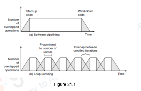
Predication: So far, we have looked at different techniques that the compiler uses to exploit ILP. Software support of ILP is best when code is predictable at compile time. But what if there’s no predictability? In such cases, the compiler cannot exploit ILP on its own and relies on the hardware to provide some support. We shall now look at such techniques. First of all, we shall discuss about predication.

Predicated or conditional instructions are provided in the ISA of the processor and the compiler uses these instructions. A predicated instruction is executed if the condition is true and annulled if the condition is false. Thus, branches can be removed and the condition that the branches tested for can be incorporated as a predicate in the instruction. A control dependence is thus transformed to a data dependence. Some architectures have a few predicated instructions, whereas, some architectures support full predication. That is, the execution of all instructions is controlled by a predicate. This feature allows us to simply convert large blocks of code that are branch dependent. When we have an if then else construct, the statements in the if section will be replaced with a predicate and all the statements in the else clause will be replaced with the opposite predicate, say zero and non-zero. This process is called if-conversion.

Predicated instructions can also be used to speculatively move an instruction that is time-critical, but may cause an exception if moved before a guarding branch. Consider the following code sequence shown in Figure 21.2 for a two-issue superscalar that can issue a combination of one memory reference and one ALU operation, or a branch by itself, every cycle. The second cycle wastes one slot and the last LW instruction has a data dependence on the previous LW. This will cause a stall if the branch is not taken.

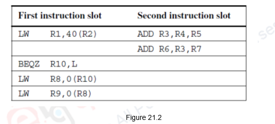
The use of predicated instructions can improve the schedule as indicated in Figure 21.3. The conditional load instruction, LWC helps in filling the slot in the second clock cycle and also avoids the stall due to data dependence for the last instruction. The conditional load is executed unless the third operand is zero. Thus, this gives a better schedule.

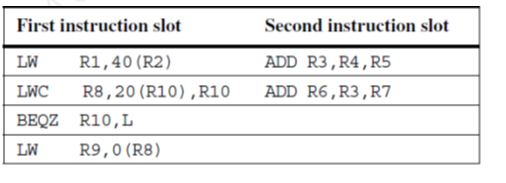
Predicated instructions have some drawbacks. They are:

- - Annulled predicated instructions also take some processor resources
  - Predicated instructions are more useful when the predicate can be evaluated early
  - The use of conditional instructions can be limited when the control flow involves more than a simple alternative sequence
  - Conditional instructions may have some speed penalty compared with unconditional instructions
  - As data dependences are normally resolved early in the pipeline, this may give rise to stalls

Software Speculation with Hardware Support: The compiler uses static prediction to predict the behaviour of branches at compile time either from the program structure or by using a profile. In such cases, the compiler may want to speculate either to improve the scheduling or to increase the issue rate. Predicated instructions provide one method to speculate, but they are really more useful when control dependences can be completely eliminated by if-conversion. However, in many cases, we would like to move speculated instructions not only before branch, but before the condition evaluation, and predication cannot achieve this.

In order to perform aggressive speculation, we need three capabilities:

The ability of the compiler to find instructions that, with the possible use of register renaming, can be speculatively moved and not affect the program data flow
The ability to ignore exceptions in speculated instructions, until we know that such exceptions should really occur, and
The ability to speculatively interchange loads and stores, or stores and stores, which may have address conflicts.

The first of these is a compiler capability, while the last two require hardware support, which we explore next.

Hardware Support for Preserving Exception Behavior: In order to speculate ambitiously, we must be able to move any type of instruction and still preserve its exception behavior. The key to being able to do this is to observe that the results of a speculated sequence that is mispredicted will not be used in the final computation, and such a speculated instruction should not cause an exception.

There are four methods that have been investigated for supporting more ambitious speculation without introducing erroneous exception behavior:

The hardware and operating system cooperatively ignore exceptions for speculative instructions. This approach preserves exception behavior for correct programs, but not for incorrect ones.
Speculative instructions that never raise exceptions are used, and checks are introduced to determine when an exception should occur.
A set of status bits, called poison bits, are attached to the result registers written by speculated instructions when the instructions cause exceptions. The poison bits cause a fault when a normal instruction attempts to use the register.
A mechanism is provided to indicate that an instruction is speculative and the hardware buffers the instruction result until it is certain that the instruction is no longer speculative.

Finally, a comparison between software and hardware speculation can be done. The comparison is provided below.

- In the case of software speculation, memory references must be disambiguated
- Hardware-based speculation works better when control flow is unpredictable
- Hardware-based speculation maintains a completely precise exception model even for speculated instructions
- Hardware-based speculation does not require compensation or bookkeeping code, unlike software speculation mechanisms
- Compiler-based approaches may benefit from the ability to see further in the code sequence, resulting in a better code scheduling than a purely hardware-driven approach
- Hardware-based speculation with dynamic scheduling does not require different code sequences to achieve good performance for different implementations of an architecture

To summarize, we have looked at how software pipelining can be implemented. It does a symbolic unrolling process, just like what Tomasulo does in hardware. We also looked at how the compiler can exploit more ILP using predicated or conditional instructions. The concept of speculation can also be used by the compiler to uncover more ILP, provided the hardware supports in preserving exception behavior and memory disambiguation.

Web Links / Supporting Materials

Computer Organization and Design – The Hardware / Software Interface, David A. Patterson and John L. Hennessy, 4th Edition, Morgan Kaufmann, Elsevier, 2009.

Computer Architecture – A Quantitative Approach , John L. Hennessy and David A. Patterson, 5th Edition, Morgan Kaufmann, Elsevier, 2011.

Multiple Issue Processors I

The objectives of this module are to discuss the need for multiple issue processors, look at the different types of multiple processors and discuss various implementation and design issues.

So far, we have looked at various hardware and software techniques to exploit ILP. The ideal CPI that we can expect in a pipelined implementation is only 1. If we want to further reduce CPI, we need to explore the option of issuing and completing multiple instructions every clock cycle. For example, if we issue and complete two instructions every clock cycle, ideally we should get a CPI of 0.5. Such processors are called multiple issue processors.

Consider the simple MIPS integer pipeline that we are familiar with. This gets extended with multiple functional units for the execution stage when we look at different types of fixed and floating point operations. We can also increase the depth of the pipeline, which may be required because of the increase in clock speeds. Now, in multiple issue processors, we increase the width of the pipeline. Several instructions are fetched and decoded in the front-end of the pipeline. Several instructions are issued to the functional units in the back-end. Suppose if m is the maximum number of instructions that can be issued in one cycle, we say that the processor is m-issue wide.

Types of Multiple Issue Processors: There are basically two variations in multiple issue processors – Superscalar processors and VLIW (Very Long Instruction Word) processors. There are two types of superscalar processors that issue varying numbers of instructions per clock. They are

statically scheduled superscalars that use in-order execution
dynamically scheduled superscalars that use out-of-order execution

VLIW processors, in contrast, issue a fixed number of instructions formatted either as one large instruction or as a fixed instruction packet with the parallelism among instructions explicitly indicated by the instruction. Hence, they are also known as EPIC–Explicitly Parallel Instruction Computers. Examples include the Intel/HP Itanium processor. A summary of the characteristics of the various types is provided in the table below.

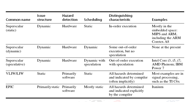
Superscalar processors decide on the fly how many instructions are to be issued. If instructions are issued to the back-end in program order, we have in-order processors. In-order processors are statically scheduled, i.e., the scheduling is done at compile-time. A statically scheduled superscalar must check for any dependences between instructions in the issue packet and any instruction already in the pipeline. They require significant compiler assistance to achieve good performance as the compiler does most of the work of finding and scheduling instructions for parallel execution. In contrast, a dynamically scheduled superscalar requires less compiler assistance, but significant hardware costs. If instructions can be issued to the back-end in any order, we have out-of-order (OOO) processors. OOO processors are dynamically scheduled by the hardware.

An alternative to superscalar approach is to rely on the compiler technology to minimize the potential stalls due to hazards. The instructions are formatted in a potential issue packet so that the hardware need not check explicitly for dependences. The compiler ensures that there are on dependences within the issue packet or indicates when a dependence occurs. This architectural approach was named VLIW. The compiler technology offers the potential advantage of having simpler hardware, while still exhibiting good performance through extensive compiler technology. We will look at details of each of these types of multiple issue processors. This module will focus on the superscalar processors and the next module will discuss the VLIW style of architectures.

Statically Scheduled Superscalar Processors: In such processors, we issue instructions in issue packets with the number of instructions ranging from 0 to 8. Suppose we consider a 4-issue superscalar, then up to four instructions will be taken from the fetch unit. The fetch unit may or may not be able to supply all the four instructions. During the issue stage, all hazards are checked in hardware (dynamic issue capability). The hazards among instructions in the issue packet as well as the ones between the instructions in the packet and the ones already in execution need be checked by the pipeline control logic. If one instruction in the packet cannot be issued, only the preceding instructions are issued. That is, we look at an in-order issue.

Hazard checks normally take a long time and if they are to be done in one clock cycle, then the issue logic decides the minimum clock cycle time. In order to avoid this, the issue stage is split into two and pipelined. The hazards among instructions in the same packet are checked in the 1st stage. The hazards among the instructions in the packet and the ones already in the pipeline are checked in the 2nd. stage.

Statically Scheduled Superscalar MIPS: Let us assume a statically scheduled superscalar MIPS and also assume that two instructions are issued per clock cycle. One of them is a floating point operation and the other is a Load/Store/Branch/ Integer operation. This is much simpler and less demanding than arbitrary dual issue.

For this processor, upto two instructions will have to be fetched every clock cycle. The hazard checking process is relatively straightforward, since the restriction of one integer and one FP instruction eliminates most hazard possibilities within the issue packet. The only difficulties that arise are when the integer instruction is a floating-point load, store, or move. This possibility creates contention for the floating-point register ports and may also create a new RAW hazard when the second instruction of the pair depends on the first. Finally, the instructions chosen for execution are dispatched to their appropriate functional units. Figure 22.1 shows how the instructions look as they go into the pipeline in pairs. Here, we assume that the floating point instruction takes three clock cycles for execution.

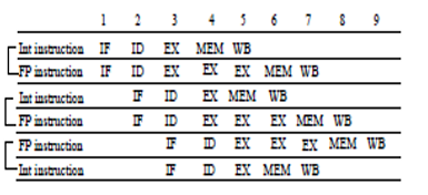
The problems of this superscalar MIPS are the following:

– Additional hardware in the pipeline
- This definitely requires more hardware than the single issue MIPS
– Out-of-order completion will lead to imprecise interrupts
- A floating point instruction can finish execution after an integer instruction that is later in program order
The floating point instruction exception could be detected after the integer instruction completed
- Several solutions like early detection of FP exceptions, the use of software mechanisms to restore a precise exception state before resuming execution, and delaying instruction completion until we know an exception is impossible
– Hazard penalties may be longer
- The result of a load instruction cannot be used on the same clock cycle or on the next clock cycle, and hence, the next three instructions cannot use the load result without stalling. The branch delay for a taken branch becomes either two or three instructions, depending on whether the branch is the first or second instruction of a pair

Dynamically Scheduled Superscalar MIPS: As we have already discussed in the earlier modules with single issue, dynamic scheduling is one method for improving performance in a multiple issue processor also. When applied to a superscalar processor, dynamic scheduling not only improves performance when there are data dependences, it also allows the processor to potentially overcome the issue restrictions. That is, although the hardware may not be able to initiate execution of more than one integer and one FP operation in a clock cycle, dynamic scheduling can eliminate this restriction at instruction issue, at least until the hardware runs out of reservation stations.

Let us assume that we want to extend the Tomasulo’s algorithm to support dual issue. Instructions will have to be issued in-order to the reservation stations. Otherwise, it will lead to a violation of the program semantics. We can assume that any combination of instructions can be issued, but this will significantly complicate instruction issue. Alternatively, we can separate the data structures for the integer and floating-point registers. Then we can simultaneously issue a floating-point instruction and an integer instruction to their respective reservation stations, as long as the two issued instructions do not access the same register set. Two different approaches have been used to issue multiple instructions per clock in a dynamically scheduled processor. They are:

Pipelining, so that two instructions can be processed in one clock cycle
Increase the logic to handle two instructions, including any possible dependences between the instructions. Modern superscalar processors that issue four or more instructions per clock often include both approaches – they both pipeline and widen the issue logic.

Let us now see how a simple loop shown below executes on this dual issue processor.

Loop: LD R2, 0(R1) ;R2=array element

DADDIU R2,R2,#1 ;increment R2

SD R2, 0(R1) ;store result

DADDIU R1,R1,#8 ;increment pointer

BNE R2,R3,LOOP ;branch if not last element

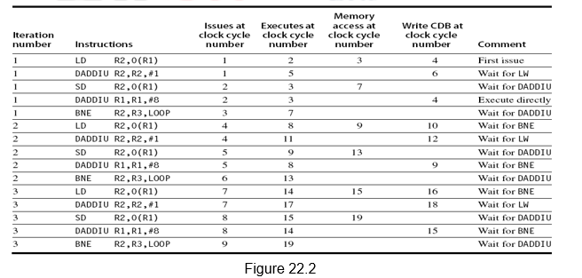
In the first clock cycle, both LD and DADDIU instructions of iteration 1 are issued. LD finishes in the fourth clock cycle and because of the dependency, DADDIU executes in 5 and writes in 6. During the second clock cycle, SD and the second DADDIU of iteration 1 are issued. SD calculates the effective address in 3, but does the memory write in 7. Branch is single-issued in clock cycle 3. The branch is resolved in 7. The LD and DADDIU of iteration 2 are issued in clock cycle 4. However, they execute only after the branch is resolved. So, LD finishes in 10, and so on. The entire schedule is given in Figure 22.2.

Dynamically Scheduled Superscalar MIPS with Speculation: The performance of the dynamically scheduled superscalar can be improved further with speculation. The concept of speculation has already been discussed with respect to single issue processors. The same is extended to multiple issue processors. Instructions beyond the branch are not only fetched and issued, but also executed. The results are put in the ROB. When the instruction is scheduled to commit, the results are written from the ROB to the register file or memory. The architecture of a dynamic scheduler with support for speculation is repeated in Figure 22.3 for ready reference. The instructions go through four steps – issue, execute, write result and commit. The complete schedule for three iterations for the same loop discussed earlier is given in Figure 22.4.

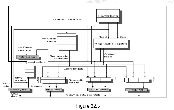
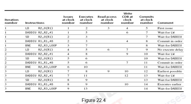
The schedule is generated as before except for the following changes:

Since it a speculative execution, a fourth stage called commit is included.
Also, since it is a speculative execution, the instructions after the Branch need not have to wait for the branch to resolve.
Note that even though the branch gets resolved only in clock cycle 7, the following LD instruction executes in clock cycle 5 itself.
Since multiple issue and execute might lead to multiple instructions finishing in the same clock cycle, two CDBs and two commits per clock cycle have been assumed.

Implementation Issues: The following points will have to be remembered while performing dynamic scheduling with speculation. We need each of the following steps to take place in 1 cycle apiece:

o Fetch some number of instructions from instruction cache and branch prediction/target buffer
- apply the prediction
- update the buffer on miss-predictions and cache misses
o Find instructions from the queue that can be issued in parallel
- Are reservation stations available for the collection of instructions?
- Is there room in the ROB?
- Handle WAW/WAR hazard through register renaming
- Move instructions to ROB
o Execute at the functional units as data become available (number of cycles varies by type of functional unit)
o Send results out on CDB if it is not currently busy
o CDB bottle neck?
o Commit the next instruction(s) in the ROB
- forwarding data to register/store units
- with the multi-issue, we might want to commit > 1 instruction per cycle or the ROB becomes a potential bottleneck

Design Issues with Speculation: There are many design issues that will have to be considered. They are discussed below.

How Much Can We Speculate?

One of the main advantages of speculation is that it will handle events that might stall the pipeline earlier, say, cache misses. However, if the processor speculates and executes a costly event like a TLB miss and later on finds that this should not have been executed, the advantage of speculation is lost. Therefore, most pipelines with speculation will allow only low-cost exceptional events (such as a first-level cache miss) to be handled in speculative mode. If an expensive exceptional event occurs, such as a second-level cache miss or a TLB miss, the processor will wait until the instruction causing the event is no longer speculative before handling the event. Although this may slightly degrade the performance of some programs, it avoids significant performance losses in others, especially those that suffer from a high frequency of such events coupled with less than excellent branch prediction.

2. Speculating Through Multiple Branches: Normally we assume that we speculate on one branch. What happens if there is another branch coming in before the earlier branch is resolved? Can we speculate across multiple branches? This becomes more complicated and is a design issue.

3. Window Size: If the issue unit must look at n instructions (n is our window size) to find those that can be issued simultaneously, it requires (n-1)2 comparisons. A window of 4 instructions would require 9 comparisons, a window of 6 instructions would require 25 comparisons. These comparisons must take place in a short amount of time so that the instructions can be issued in the same cycle and data forwarded to reservation stations and ROB. That’s a lot of work in 1 cycle! Modern processors have a window size of 2-8 instructions although the most aggressive has a window 32.

To summarize, we have looked at the need for multiple issue processors. We have discussed the different types of such processors. Statically scheduled superscalars are statically scheduled, but are dynamically issued and the hazard detection is done in hardware. On the other hand, dynamically scheduled superscalars are dynamically scheduled, with dynamic issue and the hazard detection done in hardware. We also discussed the implementation issues and design issues associated with superscalar processors. The other type of multiple issue processor, namely, VLIW will be dealt with in detail in the next module.

Web Links / Supporting Materials

Computer Organization and Design – The Hardware / Software Interface, David A. Patterson and John L. Hennessy, 4th Edition, Morgan Kaufmann, Elsevier, 2009.

Computer Architecture – A Quantitative Approach , John L. Hennessy and David A. Patterson, 5th Edition, Morgan Kaufmann, Elsevier, 2011.

Multiple Issue Processors II

The objectives of this module are to discuss in detail about the VLIW architectures and discuss the various implementation and design issues related to the VLIW style of architectures.

The previous module discussed the need for multiple issue processors. We also discussed in detail about statically scheduled and dynamically scheduled superscalars. Now, we will discuss the other type of multiple issue processors, viz., VLIW processors.

VLIW (Very Long Instruction Word) processors: In this style of architectures, the compiler formats a fixed number of operations as one big instruction (called a bundle) and schedules them. With few numbers of instructions, say 3, it is usually called LIW (Long Instruction Word). There is a change in the instruction set architecture, i.e., 1 program counter points to 1 bundle (not 1 operation). The operations in a bundle are issued in parallel. The bundles follow a fixed format and so the decode operations are done in parallel. It is assumed that there are enough FUs for the types of operations that can issue in parallel. We can also look at pipelined FUs. Example machines that follow this style include the Multiflow & Cydra 5 (8 to 16 operations) in the 1980’s, IA-64 (3 operations), Crusoe (4 operations) and TM32 (5 operations).

The main goals of the hardware design in a processor are to reduce the hardware complexity, to shorten the cycle time for better performance and to reduce power requirements. The VLIW designs reduce hardware complexity by the following features:

less multiple-issue hardware
- no dependence checking for instructions within a bundle
- can be fewer paths between instruction issue slots & FUs
simpler instruction dispatch
- no out-of-order execution, no instruction grouping
ideally no structural hazard checking logic

All this leads to reduction in hardware complexity which in turn affects the cycle time and power consumption.

Though the hardware is less complex, the compiler becomes more complicated. We need the support of the compiler to increase ILP. Since there are multiple operations packed into one bundle with the idea of keeping the functional units busy, there must be enough parallelism in a code sequence to fill the available operation slots. This parallelism is usually uncovered by using techniques like loop unrolling and software scheduling that we discussed in the previous modules, and then scheduling these instructions appropriately. If the unrolling generates straightline code, then local scheduling techniques, which operate on a single basic block can be used. On the other hand, if finding and exploiting the parallelism requires scheduling code across branches, a substantially more complex global scheduling algorithm must be used. Global scheduling algorithms are not only more complex in structure, but they must deal with significantly more complicated tradeoffs in optimization, since moving code across branches is expensive.

Trace scheduling, is one of these global scheduling techniques developed specifically for VLIWs. The details of trace scheduling are beyond the scope of this lecture. But we will at the basic concepts involved here. Trace scheduling is a way to organize the global code motion process, so as to simplify the code scheduling by incurring the costs of possible code motion on the less frequent paths. There are two steps to trace scheduling. The first step, called trace selection, tries to find a likely sequence of basic blocks whose operations will be put together into a smaller number of instructions called a trace. Loop unrolling and static branch prediction will be used so that the resultant trace is a straight-line sequence resulting from concatenating many basic blocks. Once a trace is selected, the second process, called trace compaction, tries to squeeze the trace into a small number of wide instructions. Trace compaction is code scheduling; hence, it attempts to move operations as early as it can in a sequence (trace), packing the operations into as few wide instructions (or issue packets) as possible. Predication, which is a hardware support that allows some conditional branches to be eliminated, extending the usefulness of local scheduling and enhancing the performance of global scheduling are also extensively used.

Thus, it is seen that the compiler is responsible for uncovering parallelism and also detecting hazards and hiding the latencies associated with them. Structural hazards are handled by making sure that no two operations within a bundle are scheduled to the same functional unit and no two operations are scheduled to the same memory bank. The latencies associated with memory are handled by data prefetching and by hoisting loads above stores, with support from the hardware. Data hazards are handled by ensuring that there are no data hazards among instructions in a bundle. Control hazards are dealt using predicated execution and static branch prediction.

Let us now look at a loop that we are already familiar with and see how this can be scheduled on a VLIW processor. The code below shows a thrice unrolled and scheduled code that runs in 11 clock cycles, taking 3.67 clock cycles per iteration.

1 Loop:L.D F0,0(R1)

2 L.D F6,-8(R1)

3 L.D F10,-16(R1)

4 ADD.D F4,F0,F2

5 ADD.D F8,F6,F2

6 ADD.D F12,F10,F2

7 S.D 0(R1),F4

8 S.D -8(R1),F8

9 DSUBUI R1,R1,#24

10 BNEZ R1,LOOP

11 S.D 8(R1),F12 ; 8-24 = -16

Assuming, a VLIW processor that packs two memory operations, two floating point operations and one integer or branch operation in one bundle, a probable schedule is shown below in Figure 23.1.

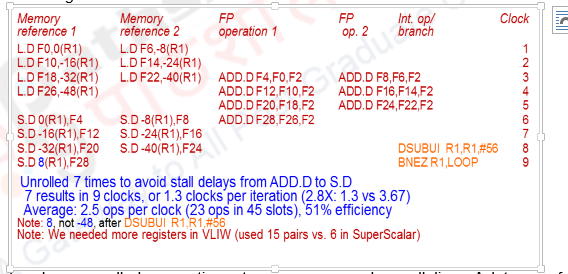
The loop has been unrolled seven times to uncover enough parallelism. A latency of one has been assumed between the Load and the Add using it, and a latency of two has been assumed between the Add and the corresponding Store. The first clock cycle issues only the two Load operations. The second clock cycle also issues only the two subsequent Loads. The third clock cycle issues two more Loads and also two Adda corresponding to the first two Loads. This is continued. Note that the first set of Stores are issued two clock cycles after the corresponding Adds. Note that the last Store uses an address 8(R1) instead of -48(R1) as the DSUBUI instruction has been moved ahead and modifies R1 by -56. This code takes 9 clock cycles for seven iterations, resulting in a rate of 1.3 clocks per iteration.

Drawbacks of the VLIW Processors: For the original VLIW model, there are both technical and logistical problems. The technical problems are the increase in code size and the limitations of the lock-step operation. The increase in code size is due to the ambitious unrolling that is done and also because of the fact that we are not able to effectively use the slots. The schedule discussed earlier itself shows that only about 60% of the functional units are used, so almost half of each instruction was empty. In most VLIWs, an instruction may need to be left completely empty if no operations can be scheduled. To handle this code size increase, clever encodings are sometimes used. For example, there may be only one large immediate field for use by any functional unit. Another technique is to compress the instructions in main memory and expand them when they are read into the cache or decoded.

Early VLIWs operated in a lock-step fashion as there was no hazard detection hardware at all. Because of this, a stall in any functional unit pipeline would cause the entire processor to stall, since all the functional units must be kept synchronized. Although a compiler may be able to schedule the deterministic functional units to prevent stalls, predicting which data accesses will encounter a cache stall and scheduling them is very difficult. Hence, caches needed to be blocking and would cause all the functional units to stall. This is too much of a restriction. In more recent processors, the functional units operate more independently, and the compiler is used to avoid hazards at issue time, while hardware checks allow for unsynchronized execution once instructions are issued.

Binary code compatibility has also been a major logistical problem for VLIWs. Different numbers of functional units and functional unit latencies require different versions of the code. This requirement makes migrating between successive implementations, or between implementations with different issue widths, more difficult than it is for a superscalar design. One possible solution to this binary code compatibility is object-code translation or emulation. This technology is developing quickly and could play a significant role in future migration schemes. Another approach is to temper the strictness of the approach so that binary compatibility is still feasible. This later approach is used in the IA-64 architecture.

Advantages of Superscalar Architectures over VLIW: When compared to the VLIW architectures, the superscalars have the following advantages:

Old codes still run without any problem
- o Like those tools you have that came as binaries
The hardware detects whether the instruction pair is a legal dual issue pair
- o If not they are run sequentially
Little impact on code density
- o You do not have to fill all the slots where you cannot issue instructions with just NOP’s
Compiler issues are very similar
- o Still need to do instruction scheduling anyway
- o Dynamic issue hardware is there so the compiler does not have to be too conservative

Explicitly Parallel Instruction Computing (EPIC) is a term coined in 1997 by the HP – Intel alliance based on the VLIW style of architectures. As VLIW processors issue a fixed number of instructions formatted as a bundle, with the parallelism among instructions explicitly indicated by the instruction, they are also known as Explicitly Parallel Instruction Computers. VLIW and EPIC processors are inherently statically scheduled by the compiler. The Itanium processor is an example of this style of architectures. The complete discussion of this architecture is beyond the scope of this discussion. However, some of the characteristics of the architecture are listed below:

Bundle of instructions
- 128 bit bundles
- 3 41-bit instructions/bundle
- 2 bundles can be issued at once
Fully predicated ISA
Registers
- 128 integer & FP registers
- 128 additional registers for loop unrolling & similar optimizations
- 8 indirect branch registers
- miscellaneous other registers
ISA & Microarchitecture seem complicated (some features of out-of-order processors)
- not all instructions in a bundle need stall if one stalls (a scoreboard keeps track of produced source operands)
- multi-level branch prediction
- register remapping to support rotating registers on the “register stack” which aid in software pipelining & dynamically sized register windows
- special hardware for “register window” overflow detection; special instructions for saving & restoring the register stack
- Speculative state cannot be stored to memory
  - special instructions check integer register poison bits to detect whether value is speculative (speculative loads or exceptions)
  - OS can override the ban (e.g., for a context switch)
  - different mechanism for floating point (status registers)
- Array address post-increment & loop control

Comparison between Superscalars and VLIW Processors: Superscalar processors have more complex hardware for instruction scheduling as they perform out-of-order execution and there are more paths between instruction issue structure and functional units. This will result in slower cycle times, more chip area and more power consumption. VLIW architectures also will have more functional units if there is support for full predication leading to the same possible consequences. VLIW architectures obviously have larger code size. The estimates of IA-64 code is up to 2X – 4X over x86. This will lead to increase in instruction bandwidth requirements and decrease in instruction cache effectiveness. They also require a more complex compiler. Superscalars can more efficiently execute pipeline-independent code. So, they do not have to recompile if we change the implementation.

To summarize, we have looked at the need for multiple issue processors. We have discussed the VLIW style of multiple issue processors. VLIW processors form instruction bundles consisting of a number of instructions and the bundles are issued statically. Hazard detection and issue are done by the compiler. The compiler has to be complicated and uses different techniques for exploiting ILP. Early VLIWs were quite rigid in their instruction formats and effectively required recompilation of programs for different versions of the hardware. To reduce this inflexibility and enhance performance of the approach, several innovations have been incorporated into more recent architectures of this type. This second generation of VLIW architectures is the approach being pursued for desktop and server markets. VLIW architectures have certain advantages and disadvantages compared to superscalar processors.

Web Links / Supporting Materials

Computer Organization and Design – The Hardware / Software Interface, David A. Patterson and John L. Hennessy, 4th Edition, Morgan Kaufmann, Elsevier, 2009.

Computer Architecture – A Quantitative Approach , John L. Hennessy and David A. Patterson, 5th Edition, Morgan Kaufmann, Elsevier, 2011.

Dynamic scheduling​

Dynamic scheduling – Example​

Dynamic scheduling – Loop Based Example​

Dynamic scheduling with Speculation​

Exploiting ILP with Software Approaches I​

Exploiting ILP with Software Approaches II​

Multiple Issue Processors I​

Multiple Issue Processors II​

Dynamic scheduling

Dynamic scheduling – Example

Dynamic scheduling – Loop Based Example

Dynamic scheduling with Speculation

Exploiting ILP with Software Approaches I

Exploiting ILP with Software Approaches II

Multiple Issue Processors I

Multiple Issue Processors II