Performance Metrics and Benchmarks

Performance Metrics

The objectives of this module are to identify and evaluate the performance metrics for a processor and also discuss the CPU performance equation.

When you look at the computer engineering methodology you have technology trends that happen and various improvements that happen with respect to technology and this will give rise to newer and newer architectures. You have to evaluate the existing systems for bottlenecks and then try to come up with better architectures and this process continues. While evaluating the existing systems for bottlenecks, you will have to have certain metrics and certain benchmarks based on which you’ll have the evaluation done.

You should basically be able to

• measure performance
• report performance and
• summarise performance.

These steps are necessary because that’ll help you make intelligent choices about the computer systems that you want to purchase. It will help you see through the marketing hype – there is so much of hype happening about computer systems and unless you have some basics about the performance of computer systems you will not be able to manage this and you will not be able to make a judicious choice when purchasing systems. Understanding performance measures is also a key to understanding the underlying organizational motivation, based on what factors people try to bring these modifications, so that performance will be improved. You will be able to understand the motivational aspects based on which certain innovations were brought in. While discussing about performance, you should be able to answer some questions like this:

• Why is some hardware better than others for different programs?

• What factors of system performance are hardware related? (e.g., Do we need a new machine, or a new operating system?)

• How does the machine’s instruction set affect performance?

Performance is important both from the purchasing perspective and the designer’s perspective. When you look at the purchasing perspective, given a collection of machines, you’ll have to be able to decide which has the best performance, the least cost, and also the best cost per performance ratio. Similarly, from a designer’s perspective, you are faced with several design options like which has the best performance improvement, least cost and best cost/performance. Unless you have some idea about the performance metrics, you will not be able to decide which will be the best performance improvement that you can think of and which will lead to least cost and which will give you the best cost performance ratio. So, whether you’re looking at the designer’s perspective or purchaser’s perspective, both of them need to have some knowledge about the performance metrics and both require these performance metrics for comparison.

Our goal is to understand what factors in the architecture contribute to the overall system performance and the relative importance and cost of these factors. Performance means different things to different people. Say, for example, take an analogy from the airline industry. If you have to choose between different types of aircrafts, what the various factors that you’ll have to consider? Do you have to worry only about the cruising speed – how fast the craft flies, or do you have to worry about how far the car craft will fly – the flight range., or look at how big these aircrafts are and how many people can be transported at one point of time from one place to another place. So these are different factors that need to be considered and you cannot expect a particular aircraft to satisfy all these requirements. You’ll have to decide which one is more important than the other factors. All three factors are important, no doubt about it, but all three of them may not be equally important – you may have more importance to certain factors compared to other factors. The criteria of performance evaluation differ among the users and designers. The same holds good when you’re looking at a computer industry also. You have different classes of computer systems and you may have certain performance criteria which are important for certain types of applications, whereas they may not be so important for other types of applications. You should be able to decide which is important for which type of processor. You’ll have to be aware of the fact that you should never let an engineer get away with simply presenting the data – you always should insist that he or she should lead off with the conclusions to which the data led, to justify the reasons why you get these data. Only when you are able to understand the internal architecture of the processor, you’ll be able to make a judicious choice.

There are different things that affect the performance of a computer system. The instructions that you use and the implementation of these instructions, the memory hierarchy, the way the I/O is handled – all this may contribute to your performance. The primary factor when you’re looking at computer performance is time. All of us are worried about how fast the program executes. So the most important performance factor is the time. When you’re looking at time being the most important factor, are you looking at response time, or are you looking at something else? What we mean by response time is the latency – you ask the processor to execute a particular task and how fast you get a response from the processor – that is basically what is called the response time.

• How long does it take for my job to run?
• How long does it take to execute a job?
• How long must I wait for the database query?

The other important time factor is throughput. It is the total amount of work done in a given time.

• How many jobs can the machine run at once?

• What is the average execution rate?

• How much work is getting done?

Response time (execution time) – the time between the start and the completion of a task is important to individual users. Throughput (bandwidth) – the total amount of work done in a given time is important to data center managers. We will need different performance metrics as well as a different set of applications to benchmark embedded and desktop computers, which are more focused on response time, versus servers, which are more focused on throughput

If we have to maximize performance, we obviously need to minimize our execution time. Performance is inversely related to execution time.

Performance = 1/ Execution time

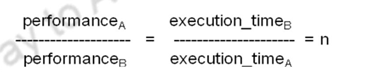
If a processor X is n times faster than Y, then,

Decreasing response time almost always improves throughput.

As an example, If computer A runs a program in 10 seconds and computer B runs the same program in 20 seconds, how much faster is A than B?

Speedup of A over B = 20 /10 = 2, indicating A is two times faster than B.

Execution time is the time the CPU spends working on the task, it does not include the time waiting for I/O or running other programs. You know the processor does not run only your program, it may be running other programs also and when there is an I/O transfer, it may block this program and then switch over to a different program. We don’t consider the time taken for doing the I/O operations and always only worried about the CPU execution time. That is the time that the CPU spends on a particular program.

To determine the CPU execution time for a program, you can find out the total number of clock cycles that the program takes and multiply it by the clock cycle time. Each program is made up of a number of instructions and each instruction takes a number of clock cycles to execute. If you find out the total number of clock cycles per program and if you know the clock cycle time for each of these clock cycles, then the CPU execution times can simply be calculated as the product of the total number of CPU clock cycles per program and these clock cycle. Because of the clock cycle time and clock rate being inversely related, this can also be written as CPU clock cycles for a program divided by the clock rate.

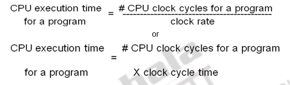
Since the CPU execution time is a product of these two factors, you can improve performance by either reducing the length of the clock cycle time or by the number of clock cycles required for a program. A clock cycle is the basic unit of time to execute one operation/pipeline stage/etc. The clock rate (clock cycles per second in MHz or GHz) is inverse of clock cycle time (clock period) CC = 1 / CR.

The clock rate basically depends on the specific CPU organization, whether it is pipelined or non-pipelined, the hardware implementation technology – the VLSI technology that is used. A 10 ns clock cycle relates to 100 MHz clock rate, a 5 ns clock cycle relates to 200 MHz clock rates and so on. If you’re looking at a 250 ps clock cycle, then it corresponds to 4 GHz clock rate. The higher the clock frequency, the lower is your clock cycle.

As an example, consider the following problem:

A program runs on computer A with a 2 GHz clock in 10 seconds. What clock rate must a computer B run at to run this program in 6 seconds? Unfortunately, to accomplish this, computer B will require 1.2 times as many clock cycles as computer A to run the program.

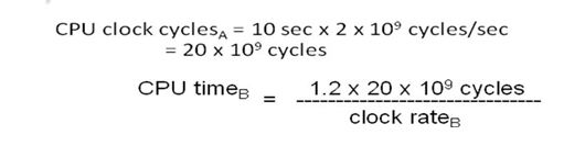
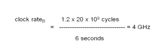
You find that the second processor should run at a clock rate of 4 GHz if you want to finish the program a little earlier.

When you have to find out the total execution time in terms of the total number of clock cycles multiplied by the clock cycle period, you have a problem of calculating the total number of clock cycles. Not all instructions take the same amount of time to execute – say you’ll have to know the number of clock cycles that each instruction takes and you should be able to add up all these clock cycles to find out the total number of clock cycles. One way to think about execution time is that it equals the number of instructions multiplied by the average time per instruction. Somehow, if we find out the average time per instruction, we should be able to calculate the execution time. A computer machine (ISA) instruction is comprised of a number of elementary or micro operations which vary in number and complexity depending on the instruction and the exact CPU organization (Design). A micro operation is an elementary hardware operation that can be performed during one CPU clock cycle. This corresponds to one micro-instruction in microprogrammed CPUs. Examples: register operations: shift, load, clear, increment, ALU operations: add , subtract, etc. Thus, a single machine instruction may take one or more CPU cycles to complete termed as the Cycles Per Instruction (CPI). Average (or effective) CPI of a program: The average CPI of all instructions executed in the program on a given CPU design.

Example problem:

• Computers A and B implement the same ISA. Computer A has a clock cycle time of 250 ps and an effective CPI of 2.0 for some program and computer B has a clock cycle time of 500 ps and an effective CPI of 1.2 for the same program. Which computer is faster and by how much?

Each computer executes the same number of instructions, I, so

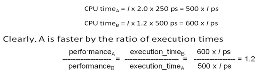
Computing the overall effective CPI is done by looking at the different types of instructions and their individual cycle counts and averaging.

where ICi is the count (percentage) of the number of instructions of class i executed, CPIi is the (average) number of clock cycles per instruction for that instruction class and n is the number of instruction classes.

The overall effective CPI varies by instruction mix – is a measure of the dynamic frequency of instructions across one or many programs.

To look at an example, consider the following instruction mix:

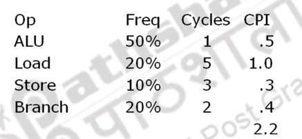
How much faster would the machine be if a better data cache reduced the average load time to 2 cycles?

–   Load à 20% x 2 cycles = .4

–   Total CPI 2.2 à 1.6

–   Relative performance is 2.2 / 1.6 = 1.38

How does this compare with reducing the branch instruction to 1 cycle?

–   Branch à 20% x 1 cycle = .2

–   Total CPI 2.2 à 2.0

– Relative performance is 2.2 / 2.0 = 1.1 We can now write the basic performance equation as:

These equations separate the three key factors that affect performance

• Can measure the CPU execution time by running the program
• The clock rate is usually given
• Can measure overall instruction count by using profilers/ simulators without knowing all of the implementation details
• CPI varies by instruction type and ISA implementation for which we must know the implementation details

To conclude, if you look at the aspects of the CPU execution time, you have three factors which affect the CPU execution time – the clock cycle time, the average number of clock cycles per instruction which is your CPI value and the instruction count. The various factors that affect these three parameters are:

• Instruction count is affected by different factors – depends on the way the program is written, if you are a skilled programmer, you use a crisp algorithm and you code it appropriately, then it is going to use less number of instructions. So, the first thing depends upon the algorithm that you want to use and the skill of the programmer who writes this code. The second thing is once you’ve written a code, the compiler is responsible for translating these instructions into your machine instructions. The compiler should be an optimizing compiler so that it translates this code into fewer number of machine instructions. The compiler definitely has a role to play in reducing the instruction count, but remember the compiler can only use the instructions that are supported in your instruction set architecture. So the instruction set architecture also plays a role in reducing the instruction count. In the previous session, we’ve looked at how the same operation can be implemented as different sequences of instructions depending upon the ISA. So with the help of the ISA, the compiler will be able to generate code which uses less number of machine instructions.
• Clock cycle time depends upon the CPU organization and also depends upon the technology that is used. By organization, we mean whether the instruction unit is implemented as a pipelined unit or a non-pipelined unit. Pipelining facilitates multi cycle operations, which reduce the clock cycle time. This will be dealt with in detail in the subsequent modules.
• CPI, which is the average number of clock cycles per instruction, depends upon the program used because you may use complicated instructions which have a number of elementary operations or simple instructions. Similarly, the compiler may translate the program using complicated instructions instead of using simpler instructions. So, the compiler may also have a role to play, and because the compiler is only using the instructions in your ISA, the ISA definitely has a role to play. Finally, the CPU organization has also a role to play in deciding the CPI values.

Having identified the various parameters that will affect the three factors constituting the CPU performance equation, computer designers should strive to take appropriate design measures to reduce these factors, thereby reducing the execution time and thus improving performance.

To summarize, we’ve looked at how we could define the performance of a processor and why performance is necessary for a computer system. We have pointed out different performance metrics, looked at the CPU performance equation and the factors that affect the CPU performance equation. This module also provided different examples which illustrate the calculation of the CPU execution time using the CPU performance equation.

Web Links / Supporting Materials

• Computer Architecture – A Quantitative Approach , John L. Hennessy and David A.Patterson, 5th.Edition, Morgan Kaufmann, Elsevier, 2011.
• Computer Organization and Design – The Hardware / Software Interface, David A. Patterson and John L. Hennessy, 4th.Edition, Morgan Kaufmann, Elsevier, 2009.
• Computer Organization, Carl Hamacher, Zvonko Vranesic and Safwat Zaky, 5th.Edition, McGraw- Hill Higher Education, 2011.

Summarizing Performance, Amdahl’s Law and Benchmarks

The objectives of this module are to discuss ways and means of reporting and summarizing performance, look at Amdahl’s law and discuss the various benchmarks for performance evaluation.

We’ve already looked at the performance equation in the earlier module. You know that the CPU execution time is the most consistent measure of performance and the CPU execution time per program is defined as the number of instructions per program multiplied by the average number of clock cycles per instruction multiplied by the clock cycle time. By improving any of these factors, by paying attention to the parameters that affect these factors, you can have an improvement in performance. Suppose you have only one processor, you can just find out the execution time with respect to that processor, with respect to a particular program, and even compare with another processor which executes the same program. But, what happens when these processors execute multiple programs? How do you summarize the performances and compare the performances? While comparing two processors, A and B, you will have to be careful in saying whether processor A is 10 times faster than or the other way round. You will have to be very careful here because wrong summary can be confusing. This module clarifies issues related to such queries.

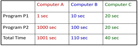
We know that the total execution time is a consistent measure of performance and the relative execution times for the same workload can also be informative. To show an example here for the importance of summarization, suppose if you have three different computer systems, which run two different programs, P1 and P2.Assume that computer A takes 1 second for executing P1 and 1000 seconds to execute P2. Similarly, B takes 10 seconds and 100 seconds respectively and c takes 20 seconds to execute both P1 and P2.

If you look at the individual performances,

• A is 10 times faster than B for program P1

• A is 20 times faster than C for program P1

• B is 10 times faster than A for program P2

• B is  2 times faster than  C for program P1

• C is 50 times faster than A for program P2

• C is 5 times faster than B for program P2

How do you summarize and say which computer is better? You can calculate the total execution time as 1001 seconds, 110 seconds and 40 seconds and based on these values, you can make the following conclusions:

• Using total execution time:

–   B is 9.1 times faster than A

–   C is 25 times faster than A

–   C is 2.75 times faster than B

If you want a single number to summarize performance, you can take the average of the execution timesand try to come up with one value which will summarize the performance. The average execution time is the summation of all the times divided by the total number of programs. For the given example, we have

Avg(A) = 500.5

Avg(B) = 55

Avg(C) = 20

Here again, if you’re trying to make a judgementbased on this, you have a problem because you know that P1 and P2 are not run equal number of times. So that may mislead your summary. Therefore, you could assign weights per program. Weighted arithmetic mean summarizes performance while tracking the execution time. Weights can adjust for different running times, balancing the contribution of each program.

One more issue that has to be mentioned before we go deeper into summarization of performance is the question of the types of programs chosen for evaluation. Each person can pick his own programs and report performance. And this is obviously not correct. So, we normally look at a set of programs, a benchmark suite to evaluate performance. Later in this module, we shall discuss in detail about benchmarks. One of the most popular benchmarks is the SPEC (Standard Performance Evaluation Corporation) benchmark. So the evaluation of processors is done with respect to this.

Even with the benchmark suite, and considering weighted arithmetic mean, the problem would be how to pick weights; since SPEC is a consortium of competing companies, each company might have their own favorite set of weights, which would make it hard to reach consensus. One approach is to use weights that make all programs execute an equal time on some reference computer, but this biases the results to the performance characteristics of the reference computer.

Rather than pick weights, we could normalize execution times to a referencecomputer by dividing the time on the reference computer by the time on the computerbeing rated, yielding a ratio proportional to performance. SPEC uses thisapproach, calling the ratio the SPECRatio. For example, suppose that theSPECRatio of computer A on a benchmark was 1.25 times higher than computerB; then you would know,

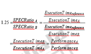
Also observe that the execution times on the reference computer drop out and thechoice of the reference computer is irrelevant when the comparisons are made asa ratio.Because a SPECRatio is a ratio rather than an absolute execution time, themean must be computed using the geometric mean. (Since SPECRatios have nounits, comparing SPECRatios arithmetically is meaningless.) The formula is

Using the geometricmean ensures two important properties:

1.  The geometric mean of the ratios is the same as the ratio of the geometricmeans.

2.  The ratio of the geometric means is equal to the geometric mean of the performance ratios, which implies that the choice of the reference computer isirrelevant.

Hence, the motivations to use the geometric mean are substantial, especiallywhen we use performance ratios to make comparisons.

Now that we have seen how to define, measure, and summarize performance, we shall explore certain guidelines and principles that areuseful in the design and analysis of computers. This section introduces importantobservations about design, as well as an important equation to evaluate alternatives. The most important observations are:

1. Take advantage of parallelism : We have already discussed the different types of parallelism that exist in applications and how architecture designers should exploit them. To mention a few – having multiple processors, having multiple threads of execution, having multiple execution units to exploit the data level parallelism, exploiting ILP through pipelining.

2. Principle of Locality: This comes from the properties of programs. A widely held rule of thumb is that a program spends 90% of its execution time in only 10% of the code. This implies that we can predict with reasonable accuracy what instructions and data a program will use in the near future based on its accesses in the recent past. Two different types of locality have been observed. Temporal locality states that recently accessed items are likely to be accessed in the near future. Spatial locality says that items whose addresses are near one another tend to be referenced close together in time.

3. Focus on the common case: This is one of the most important principles of computer architecture. While making design choices among various alternatives, always favour the most frequent case. Focusing on the common case works for power as well as for resource allocationand performance. For example, when performing the addition of two numbers, there might be overflow, but obviously not so frequent. Optimize the addition operation without overflow. When overflow occurs, it might slow down the processor, but it is only a rare occurrence and you can afford it.

In applying the simple principle of focusing on the common cases, we have to decide what the frequent case is and how much performancecan be improved by making that case faster. A fundamental law, calledAmdahl’s Law, can be used to quantify this principle.Gene Amdahl, chief architect of IBM’s first mainframe series and founder of Amdahl Corporation and other companies found that there were some fairly stringent restrictions on how much of a speedup one could get for a given enhancement. These observations were wrapped up in Amdahl’s Law. It basically states that the performance enhancement possible with a given improvement is limited by the amount that the improved feature is used. For example, you have a floatingpoint unit and you try to speed up the floatingpoint unit many times, say a 10 X speedup, but all this is going to matter only the if the floatingpoint unit is going to be used very frequently. If your program does not have floatingpoint instructions at all, then there is no point in increasing the speed of the floatingpoint unit.

The performance gain from improving some portion of  a computer is calculated by:

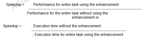
Amdahl’s Law gives us a quick way to find the speedup from some enhancement,which depends on two factors:

1. The fraction of the computation time in the original computer that can be converted to take advantage of the enhancement – For example, if 30 seconds of the execution time of a program that takes 60 seconds in total can use an enhancement, the fraction is 30/60. This value, which we will call Fractionenhanced, is always less than or equal to 1.

2. The improvement gained by the enhanced execution mode; that is, how much faster the task would run if the enhanced mode were used for the entire program – This value is the time of the original mode over the time of the enhanced mode. If the enhanced mode takes, say, 3 seconds for a portion of the program, while it is 6 seconds in the original mode, the improvement is 6/3. We will call this value, which is always greater than 1, Speedupenhanced.

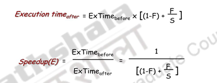
That is, suppose you define an enhancement that accelerates a fraction F of the execution time by a factor S and the remainder of the time is unaffected, then you can say, execution time with the enhancement is equal to 1 minus F, where F is the fraction of the execution time for which the enhancement is active, plus F by S, multiplied by the execution time without the enhancement. Speedup is going to be execution time without the enhancement divided by the execution time with enhancement. This is as shown above.

Amdahl’s Law can serve as a guide to how much an enhancement willimprove performance and how to distribute resources to improve cost – performance.The goal, clearly, is to spend resources proportional to where timeis spent. Amdahl’s Law is particularly useful for comparing the overall systemperformance of two alternatives, but it can also be applied to compare two processordesign alternatives.

Consider the following example to illustrate Amdahl’s law.

For the RISC machine with the following instruction mix:

CPI = 2.2

If a CPU design enhancement improves the CPI of load instructions from 5 to 2, what isthe resulting performance improvement from this enhancement?

Fraction enhanced = F =  45% or  .45

Unaffected fraction = 1- F = 100% – 45% = 55% or .55

Factor of enhancement = S =  5/2 =  2.5

Using Amdahl’s Law:

You can also alternatively calculate using the CPU performance equation.

Old CPI = 2.2

New CPI =  .5 x 1 + .2 x 2 +  .1 x 3 + .2 x 2  = 1.6

Speed up = 2.2 / 1.6 = 1.37

which is the same speedup obtained from Amdahl’s Law.

The same concept can be extended even when there are multiple enhancements. Suppose three CPU performance enhancements are proposed with the following speedups and percentage of the code execution time affected:

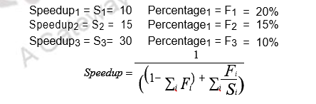
While all three enhancements are in place in the new design, each enhancement affects a different portion of the code and only one enhancement can be used at a time. What is the resulting overall speedup?

Observe that:

• The performance of any system is constrained by the speed or capacity of the slowest point.

• The impact of an effort to improve the performance of a program is primarily constrained by the amount of time that the program spends in parts of the program not targeted by the effort

The last concept that we discuss in this module is about benchmarks. To evaluate the performance of a computer system, we need a standard set of programs. Individuals cannot use their own programs that will favour their design enhancements and report improvements. So benchmarks are a set of programs that form a “workload” specifically chosen to measure performance. One of the most successful attempts to create standardized benchmark applicationsuites has been the SPEC (Standard Performance Evaluation Corporation),which had its roots in the late 1980s efforts to deliver better benchmarks forworkstations. SPEC is a non-profit corporation formed to establish, maintain and endorse a standardized set of relevant benchmarks that can be applied to the newest generation of high-performance computers. SPEC develops benchmark suites and also reviews and publishes submitted results from the member organizations and other benchmark licensees.Just as the computer industry has evolved over time, so has theneed for different benchmark suites, and there are now SPEC benchmarks tocover different application classes. All the SPEC benchmark suites and theirreported results are found at www.spec.org*.*The SPEC CPU suite is useful for processor benchmarking forboth desktop systems and single-processor servers.SPEC creates standard sets of benchmarks starting with SPEC89. The latest is SPEC CPU2006 which consists of 12 integer benchmarks (CINT2006) and 17 floating-point benchmarks (CFP2006).

The guiding principle of reporting performance measurements should be reproducibility – list everything another experimenter would need to duplicate theresults. A SPEC benchmark report requires an extensive description of the computerand the compiler flags, as well as the publication of both the baseline andoptimized results. In addition to hardware, software, and baseline tuning parameterdescriptions, a SPEC report contains the actual performance times, shownboth in tabular form and as a graph.

There are also benchmark collections for power workloads(SPECpower_ssj2008), for mail workloads (SPECmail2008), for multimedia workloads (mediabench), virtualization, etc. The following programs or benchmarks are used to evaluateperformance:

–   Actual Target Workload:  Full applications that run on the target machine.

–   Real Full Program-based Benchmarks:

• Select a specific mix or suite of programs that are typical of targeted applications or workload (e.g SPEC95, SPEC CPU2000).

–   Small “Kernel” Benchmarks:

• Key computationally-intensive pieces extracted from real programs.

–   Examples: Matrix factorization, FFT, tree search, etc.

• Best used to test specific aspects of the machine.

–   Microbenchmarks:

    • Small, specially written programs to isolate a specific aspect of performance characteristics: Processing: integer, floating point, local memory, input/output, etc.

Each of these have their merits and demerits. So, it is always a suite of programs that is chosen so that the disadvantages of one will be outweighed by the advantages of the other.

Do we have other methods of evaluating the performance, instead of the execution time? Can we consider MIPS (Millions of Instructions Per Second) as a performance measure?

For a specific program running on a specific CPU, the MIPS rating is a measure of how many millions of instructions are executed per second:

MIPS  Rating =  Instruction count /  (Execution Time x 106)

=  Instruction count  /  (CPU clocks x Cycle time x 106)

=  (Instruction count  x Clock rate)  /  (Instructioncount  x CPI x 106)

=     Clock rate  /  (CPI x 106)

There are however three problems with MIPS:

– MIPS does not account for instruction capabilities

– MIPS can vary between programs on the same computer

– MIPS can vary inversely with performance

Then, under what conditions can the MIPS rating be used to compare performance of different CPUs?

• The MIPS rating is only valid to compare the performance of different CPUs provided that the following conditions are satisfied:

1.  The same program is used

(actually this applies to all performance metrics)

2. The same ISA is used

3. The same compiler is used

(Thus the resulting programs used to run on the CPUs and obtain the MIPS rating are identical at the machine code level including the same instruction count)

So, MIPS is not a consistent measure of performance and the CPU execution time is the only consistent measure of performance.

Last of all, we should also understand that designing for performance only without considering cost and power is unrealistic

– For supercomputing performance is the primary and dominant goal

– Low-end personal and embedded computers are extremely cost driven and power sensitive

The art of computer design lies not in plugging numbers in a performance equation, but in accurately determining how design alternatives will affect performance and cost and power requirements.

To summarize, we have looked at the ways and means of summarizing performance, pointed out various factors to be considered while designing computer systems, looked at Amdahl’s law, examples for quantifying the performance, the need for and the different types of benchmarks, and last of all other metrics for performance evaluation.

Web Links / Supporting Materials

• Computer Architecture – A Quantitative Approach, John L. Hennessy and David A.Patterson, 5th.Edition, Morgan Kaufmann, Elsevier, 2011.
• Computer Organization and Design – The Hardware / Software Interface, David A. Patterson and John L. Hennessy, 4th.Edition, Morgan Kaufmann, Elsevier, 2009.
• http://en.wikipedia.org/wiki/