Arithmetic Unit

Fixed Point Arithmetic Unit I

The objectives of this module are to discuss the operation of a binary adder / subtractor unit and calculate the delays associated with this circuit, to show how the addition process can be speeded up using fast addition techniques, and to discuss the operation of a binary multiplier.

Ripple carry addition

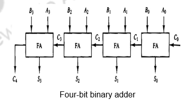
The digital circuit that generates the arithmetic sum of two binary numbers of length n is called an n-bit binary adder. It is constructed with n full-adder circuits connected in cascade, with the output carry from one full-adder connected to the input carry of the next full-adder. The Figure below shows the interconnections of four full-adders (FAs) to provide a 4-bit binary adder. The input carry to the binary adder is C0 and the output carry is C4. The S outputs of the full-adders generate the required sum bits. The n data bits for the A inputs come from one register (such as R1), and the n data bits for the B inputs come from another register (such as R2). The sum can be transferred to a third register or to one of the source registers (R1 or R2), replacing its previous content.

Binary Adder-Subtractor

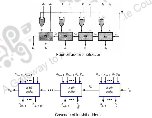
The subtraction of binary numbers can be done most conveniently by means of complements. The addition and subtraction operations can be combined into one common circuit by including an exclusive-OR gate with each full-adder. A 4-bit adder-subtractor circuit is shown in Figure. The mode input M controls the operation. When $M = 0$, the circuit is an adder and when M = 1, the circuit becomes a subtractor. Each exclusive-OR gate receives input M and one of the inputs of B. When M = 0, we have B XOR 0 = B. The full adders receive the value of B, the input carry is 0, and the circuit performs A plus B. When M =1, we have B XOR 1=B’ and C0 = 1. The B inputs are all complemented and a 1 is added through the input carry. The circuit performs the operation A plus the 2’s complement of B. For unsigned numbers, this gives $A – B$ if $A \geq B$ or the 2’s complement of (B-A) if $A<B$. For signed numbers, the result is A – B provided there is no overflow.

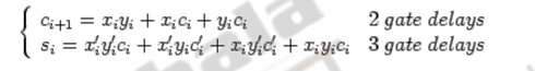
If you have to construct adders of larger sizes, these n-bit adder blocks can be cascaded as shown above.

Now, let us calculate the delay associated in doing a basic operation like addition. We know that combinational logic circuits can’t compute the outputs instantaneously. There is some delay between the time the inputs are sent to the circuit, and the time the output is computed. Let’s say the delay is T units of time. Suppose you want to implement an n-bit ripple carry adder. How much total delay is there? Since an n-bit ripple carry adder consists of n adders, there will be a delay of nT. This is O(n) delay. Why is there this much delay? After all, aren’t the adders working in parallel? While the adders are working in parallel, the carries must “ripple” their way from the least significant bit and work their way to the most significant bit. It takes T units for the carry out of the rightmost column to make it as input to the adder in the next to rightmost column. Thus, the carries slow down the circuit, making the addition linear with the number of bits in the adder. For example, consider the expressions for the sum and the carry.

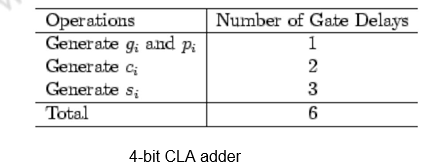
The carry takes two delays (a sum of products expression) and the sum takes three delays (one additional delay for the complement). Thus, as n increases, the delays become very high. Total time for computing the final n-bit sum from is 2(n-1) + 3 gate delays. When, n = 64, there will be 129 gate delays.

There are two ways to make the adder add more quickly. One is to go in for better technology, which again has its own limitations. The second option is to use more logic as discussed below.

Fast adders: Carry look-ahead adders

Carry lookahead adders add much faster than ripple carry adders. They do so by making some observations about carries. The bottle neck for ripple carry addition is the calculation of ci, which takes linear time proportional to n, the number of bits in the adder. To improve, we define gi, the generate function as gi = xi yi and pi, the propogate function as pi = xi + yi.

If gi  = 1, the ith bit generates a carry, ci+1 = 1.

If pi  = 1, the ith bit propagates a carry ci from (i-1)th bit to (i+1)th bit ci+1.

Both gi and pi can be generated for all n bits in constant time (1 gate delay).

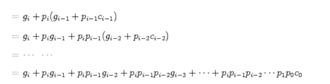
ci+1 is either generated in the ith bit (gi = 1), or propagated from the (i-1)th bit (ci = 1 and pi = 1) (maybe both).

Now all ci’s can be generated in constant time (independent of n) of 2 more gate delays after gi’s and pi’s are available. This is illustrated below.

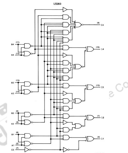
The above figure shows the logic diagram of the MSI chip 74×283 for a 4-bit adder All carries can be generated by the carry-look-ahead logic in 2 gate delays after gi’s and pi’s are available, and all sum bits can be made available in constant time of 6 gate delays, independent of number of bits in the adder.

Two-level carry look-ahead : The carry look-ahead adder requires AND and OR gates with as many as (n + 1) inputs, which is impractical in hardware realization. To compromise, we pack n =4 bits as a block with carry look-ahead, and still use ripple carry between the blocks.

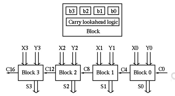
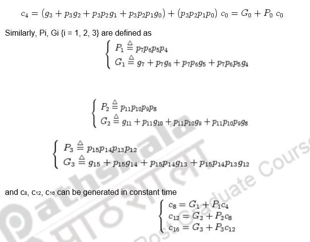
There are n / 4 blocks in an n-bit adder and the total gate delays can be found as:

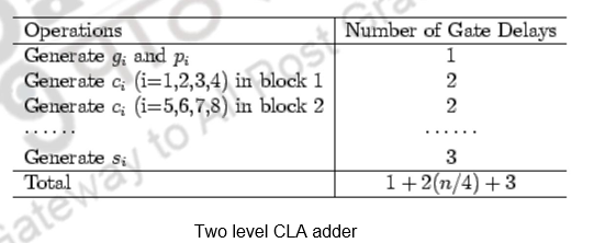
When n = 64, the number of gate delays is 36. To improve the speed further using the same idea, define 2nd-level generate and propagate functions:

P0 = p3p2p1p0

If all 4 bits in a block propagate, the block propagates a carry.

G0 = g3 + p3g2 + p3p2g1 + p3p2p1g0

If at least one of the 4 bits generates carry and it can be propagated to the MSB, the block generates a carry. Now c4 can be generated in constant time (independent of n):

Combining 4 blocks of 4-bit carry-lookahead adder as a super block, we get a 16-bit adder with 2 levels of carry-lookahead logic.

There are n / 16 super blocks in an n-bit adder and the total gate delays can be found as:

When n = 64, the number of gate delays is 14.

The very same idea can be carried out to the third level so that the carries, c16, c32, c48, and c64 can be generated simultaneously by the 3rd level carry-look ahead logic:

Binary multiplication

Multiplication of positive numbers

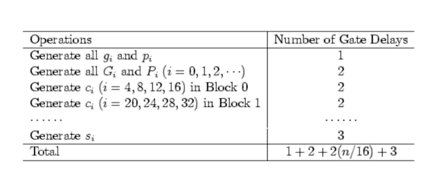
The manual multiplication algorithm carried out by hand and applicable to unsigned or positive numbers is illustrated below. Each bit of the multiplier is examined and either 0’s or the multiplicand are entered in each row, depending on the examined multiplier bit being a 0 or a 1, respectively.

The same multiplication can be implemented using combinational logic alone as shown below.

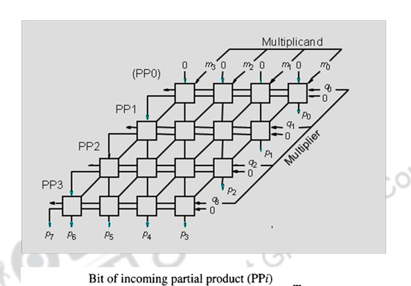
The basic cell has an AND gate which passes on 0 or the multiplicand bit, depending on whether the multiplier bit is a 0 or a 1. The full adder adds the multiplicand / 0, carry in and the partial product bit from above. Note the arrangement of this multiplier is similar in structure to the manual algorithm indicated earlier.

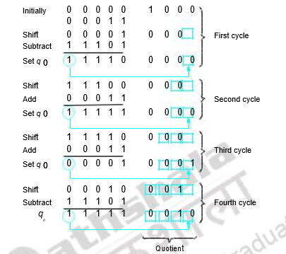
Multiplication can also be carried out using both combinational and sequential techniques. The adder in the ALU unit can be used sequentially. The algorithm, example and register organization are illustrated below.

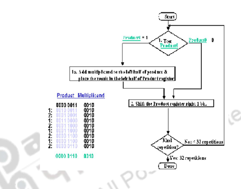
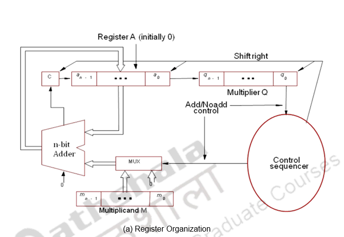
Register A is initially loaded with all 0’s, Q with the multiplier and M, with the multiplicand. The final double length product is loaded in A, Q. the control sequencer checks the LSB of the multiplier and gives the ADD / NOADD control signal. The MUX passes on the multiplicand or 0’s depending on the LSB bit. After the addition the product is shifted right, thus shifting out the checked multiplier bit and bringing in the next bit to be tested to the LSB position. This sequence is continued n times and the final product is available in A, Q. The simulation is given above.

The above technique holds good only for positive numbers. For negative numbers, the easiest way of handling is to treat the sign bits separately and attach the sign of the product finally. The other option for a negative multiplicand is to sign extend the 2’s complement of the negative multiplicand and carry out the usual process. But, if the multiplier is negative, this technique doe not work. So, the option is to complement both the numbers and then handle the negative multiplicand and positive multiplier.

There is yet another uniform method of handling positive as well as negative numbers. You will see that in the next module.

To summarize, we have discussed the fixed point arithmetic unit. We looked at binary addition, subtraction, fast adders – carry look ahead adders and binary multiplication techniques.

Web Links / Supporting Materials

• Computer Organization, Carl Hamacher, Zvonko Vranesic and Safwat Zaky, 5th.Edition, McGraw- Hill Higher Education, 2011.
• Computer Organization and Design – The Hardware / Software Interface, David A. Patterson and John L. Hennessy, 4th.Edition, Morgan Kaufmann, Elsevier, 2009.

Fixed Point Arithmetic Unit II

The objectives of this module are to discuss Booth’s multiplication technique, fast multiplication techniques and binary division techniques.

Booth’s Multiplier

The major advantage of the Booth’s technique as proposed by Andrew D. Booth is that it handles both positive and negative numbers. It may also have an added advantage of reducing the number of operations depending on the multiplier. The principle behind this is given below.

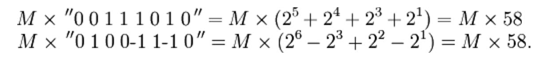
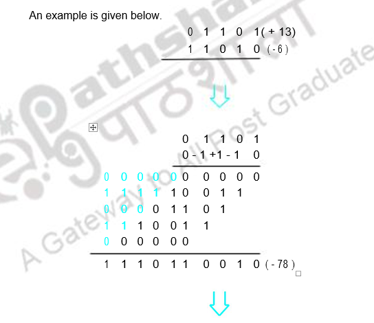
Consider a positive multiplier consisting of a block of 1s surrounded by 0s. For example, 00111110. The product is given by :

M x 00111110 = M x (2⁵ + 2⁴+ 2³ + 2² + 2¹) = M x 62, where M is the multiplicand. The number of operations can be reduced to two by rewriting the same as

M x 01000010 = M x (2⁶ – 2¹) = M x 62

In fact, it can be shown that any sequence of 1’s in a binary number can be broken into the difference of two binary numbers:

Hence, we can actually replace the multiplication by the string of ones in the original number by simpler operations, adding the multiplier, shifting the partial product thus formed by appropriate places, and then finally subtracting the multiplier. It is making use of the fact that we do not have to do anything but shift while we are dealing with 0s in a binary multiplier, and is similar to using the mathematical property that 99 = 100 − 1 while multiplying by 99.

This scheme can be extended to any number of blocks of 1s in a multiplier (including the case of single 1 in a block). Thus,

Booth’s algorithm follows this scheme by performing an addition when it encounters the first digit of a block of ones (0 1) and a subtraction when it encounters the end of the block (1 0). This works for a negative multiplier as well. When the ones in a multiplier are grouped into long blocks, Booth’s algorithm performs fewer additions and subtractions than the normal multiplication algorithm.

As a ready reference, use the table below: 

Fast multiplication

We saw the binary multiplication techniques in the previous section. This section will introduce you to two ways of speeding up the multiplication process. The first method is a further modification to the Booth’s technique that helps reduce the number of summands to n / 2 for n-bit operands. The second techinque reduces the time taken to add the summands.

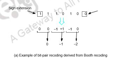
Bit – pair recoding of multiplier

This is derived from the Booth’s algorithm. It pairs the multiplier bits and gives one multiplier bit per pair, thus reducing the number of summands by half. This is shown below.

Multiplication requiring only n/2

summands Carry-save addition of summands

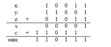
Carry save adders (CSA) speed up the addition of the summands generated during the multiplication process. The inputs to a full adder are normally the two bits of the two numbers and the carry input from the previous stage. On the other hand, in the case of the CSA, all the three bits are taken from the three numbers. The carry generated is saved and added at the next level. A CSA takes in two inputs and outputs two outputs. This is shown below.

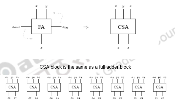
As the figure above shows, one CSA block is used for every bit. This circuit adds 3 8-bit numbers into two numbers.

The important point is that c and s can be computed independently and each ci and si can be computed independent of all other ci’s and si’s. An example is given below.

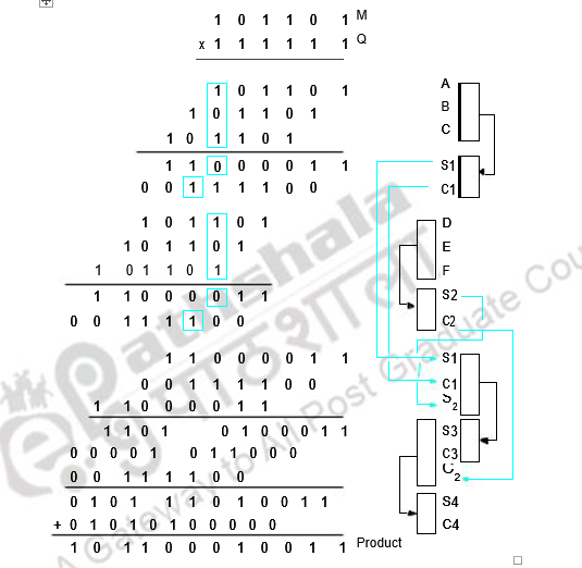
The multiplication process carried out using CSA is illustrated below.

Thus, in order to speed up the multiplication process, bit-pair recoding of the multiplier is used to reduce the summands. These summands are then reduced to 2 using a few CSA steps. The final product is generated by an addition operation that uses CLA. All these three techniques help in reducing the time taken for multiplication.

Binary division

An example of binary division is shown below. We first examine the divisor and the dividend, decide that only if we consider the first three bits of the dividend the divisor will go and then proceed. The first two bits, though not shown, will have to be 0’s. We then get a quotient bit of 1, do the subtraction, get the partial remainder and do the trial subtraction (mentally) and accordingly generate the quotient bit. This process is repeated till we exhaust all the dividend bits. This is illustrated below.

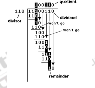
Now, the same logic has to be adopted for machine implementation too. Only thing is that, it has to be done systematically, and to decide whether the divisor is less than or equal to the dividend, we have to do a trial comparison / subtraction. There are basically two types of division algorithms:

• Restoring division
• Non-restoring division

Both these are for positive numbers. Negative numbers are handled the same way with the sign bits processed separately.

Restoring division

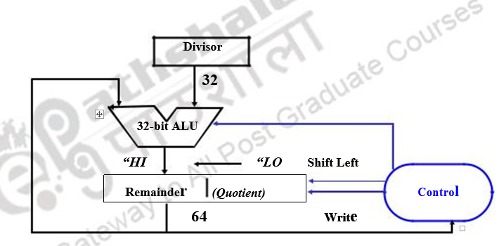
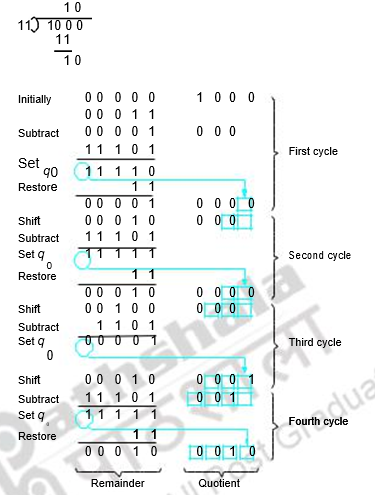
Take the first bit of the dividend and do a trial subtraction. If the subtraction produces a negative result, we generate a quotient bit of zero, restore, bring the next bit of dividend and continue. Otherwise, we simply continue with a quotient bit of 1. The algorithm, register organization and example are given below.

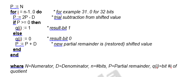
where N=Numerator, D=Denominator, n=#bits, P=Partial remainder, q(i)=bit #i of quotient

Non-restoring division

This is a modification of the restoring algorithm. It combines the restore / no restore and shift left steps of two successive cycles and reduces the number of operations. The algorithm is given below.

• Do the first shift and subtraction
• Check sign of the partial remainder
• If it is negative, shift and add
• If it is positive, shift and subtract
• Fix the quotient bit appropriately
• If the final remainder is negative, add the divisor**.**

An example is discussed below.

Remainder

To summarize, we have discussed the Booth’s multiplication technique used for handling positive and negative numbers in the same manner. We also discussed carry save addition and saw how fast multiplication can be carried out. Finally, we discussed the restoring and non restoring division algorithms.

Web Links / Supporting Materials

• Computer Organization, Carl Hamacher, Zvonko Vranesic and Safwat Zaky, 5th.Edition, McGraw- Hill Higher Education, 2011.
• Computer Organization and Design – The Hardware / Software Interface, David A. Patterson and John L. Hennessy, 4th.Edition, Morgan Kaufmann, Elsevier, 2009.

Floating Point Arithmetic Unit

The objectives of this module are to discuss the need for floating point numbers, the standard representation used for floating point numbers and discuss how the various floating point arithmetic operations of addition, subtraction, multiplication and division are carried out.

Floating-point numbers and operations

Representation

When you have to represent very small or very large numbers, a fixed point representation will not do. The accuracy will be lost. Therefore, you will have to look at floating-point representations, where the binary point is assumed to be floating. When you consider a decimal number 12.34 * 107, this can also be treated as 0.1234 * 109, where 0.1234 is the fixed-point mantissa. The other part represents the exponent value, and indicates that the actual position of the binary point is 9 positions to the right (left) of the indicated binary point in the fraction. Since the binary point can be moved to any position and the exponent value adjusted appropriately, it is called a floating-point representation. By convention, you generally go in for a normalized representation, wherein the floating-point is placed to the right of the first nonzero (significant) digit. The base need not be specified explicitly and the sign, the significant digits and the signed exponent constitute the representation.

The IEEE (Institute of Electrical and Electronics Engineers) has produced a standard for floating point arithmetic. This standard specifies how single precision (32 bit) and double precision (64 bit) floating point numbers are to be represented, as well as how arithmetic should be carried out on them. The IEEE single precision floating point standard representation requires a 32 bit word, which may be represented as numbered from 0 to 31, left to right. The first bit is the sign bit, S, the next eight bits are the exponent bits, ‘E’, and the final 23 bits are the fraction ‘F’. Instead of the signed exponent E, the value stored is an unsigned integer E’ = E + 127, called the excess-127 format. Therefore, E’ is in the range 0 £ E’ £ 255.

S E’E’E’E’E’E’E’E’ FFFFFFFFFFFFFFFFFFFFFFF

0 1                                     8  9                                                                    31

The value V represented by the word may be determined as follows:

• If E’ = 255 and F is nonzero, then V = NaN (“Not a number”)
• If E’ = 255 and F is zero and S is 1, then V = -Infinity
• If E’ = 255 and F is zero and S is 0, then V = Infinity
• If 0 < E< 255 then V =(-1)**S * 2 ** (E-127) * (1.F) where “1.F” is intended to represent the binary number created by prefixing F with an implicit leading 1 and a binary point.
• If E’ = 0 and F is nonzero, then V = (-1)**S * 2 ** (-126) * (0.F). These are “unnormalized” values.
• If E’= 0 and F is zero and S is 1, then V = -0
• If E’ = 0 and F is zero and S is 0, then V = 0

For example,

0 00000000 00000000000000000000000 = 0

1 00000000 00000000000000000000000 = -0

0 11111111 00000000000000000000000 = Infinity

1 11111111 00000000000000000000000 = -Infinity

0 11111111 00000100000000000000000 = NaN

1 11111111 00100010001001010101010 = NaN

0 10000000 00000000000000000000000 = +1 * 2**(128-127) * 1.0 = 2

0 10000001 10100000000000000000000 = +1 * 2**(129-127) * 1.101 = 6.5

1 10000001 10100000000000000000000 = -1 * 2**(129-127) * 1.101 = -6.5

0  00000001 00000000000000000000000 = +1 * 2**(1-127) * 1.0 = 2**(-126)

0  00000000 10000000000000000000000 = +1 * 2**(-126) * 0.1 = 2**(-127)

0  00000000 00000000000000000000001 = +1 * 2**(-126) *

0.00000000000000000000001 = 2**(-149) (Smallest positive value)

(unnormalized values)

Double Precision Numbers:

The IEEE double precision floating point standard representation requires a 64-bit word, which may be represented as numbered from 0 to 63, left to right. The first bit is the sign bit, S, the next eleven bits are the excess-1023 exponent bits, E’, and the final 52 bits are the fraction ‘F’:

S  E’E’E’E’E’E’E’E’E’E’E’

FFFFFFFFFFFFFFFFFFFFFFFFFFFFFFFFFFFFFFFFFFFFFFFFFFFF

0 1                                                     11 12

63

The value V represented by the word may be determined as follows:

• If E’ = 2047 and F is nonzero, then V = NaN (“Not a number”)
• If E’= 2047 and F is zero and S is 1, then V = -Infinity
• If E’= 2047 and F is zero and S is 0, then V = Infinity
• If 0 < E’< 2047 then V = (-1)**S * 2 ** (E-1023) * (1.F) where “1.F” is intended to represent the binary number created by prefixing F with an implicit leading 1 and a binary point.
• If E’= 0 and F is nonzero, then V = (-1)**S * 2 ** (-1022) * (0.F) These are “unnormalized” values.
• If E’= 0 and F is zero and S is 1, then V = – 0
• If E’= 0 and F is zero and S is 0, then V = 0

Arithmetic unit

Arithmetic operations on floating point numbers consist of addition, subtraction, multiplication and division. The operations are done with algorithms similar to those used on sign magnitude integers (because of the similarity of representation) — example, only add numbers of the same sign. If the numbers are of opposite sign, must do subtraction.

ADDITION

Example on decimal value given in scientific notation:

3.25 x 10 ** 3

+ 2.63 x 10 ** -1

—————–

    first step: align decimal points

second step: add

3.25       x 10 ** 3

+  0.000263 x 10 ** 3

——————–

3.250263 x 10 ** 3

(presumes use of infinite precision, without regard for accuracy)

third step:  normalize the result (already normalized!)

Example on floating pt. value given in binary:

.25 =    0 01111101 00000000000000000000000

 100 =    0 10000101 10010000000000000000000

To add these fl. pt. representations,

step 1:  align radix points

shifting the mantissa left by 1 bit decreases the exponent by 1

shifting the mantissa right by 1 bit increases the exponent by 1

we want to shift the mantissa right, because the bits that fall off the end should come from the least significant end of the mantissa

-> choose to shift the .25, since we want to increase it’s exponent.

-> shift by  10000101

-01111101

———

00001000    (8) places.

0 01111101 00000000000000000000000 (original value)

0 01111110 10000000000000000000000 (shifted 1 place)

(note that hidden bit is shifted into msb of mantissa)

0 01111111 01000000000000000000000 (shifted 2 places)

0 10000000 00100000000000000000000 (shifted 3 places)

0 10000001 00010000000000000000000 (shifted 4 places)

0 10000010 00001000000000000000000 (shifted 5 places)

0 10000011 00000100000000000000000 (shifted 6 places)

0 10000100 00000010000000000000000 (shifted 7 places)

0 10000101 00000001000000000000000 (shifted 8 places)

step 2: add (don’t forget the hidden bit for the 100)

0 10000101 1.10010000000000000000000  (100)

+    0 10000101 0.00000001000000000000000  (.25)

—————————————

0 10000101 1.10010001000000000000000

step 3:  normalize the result (get the “hidden bit” to be a 1)

It already is for this example.

result is

0 10000101 10010001000000000000000

SUBTRACTION

Same as addition as far as alignment of radix points

Then the algorithm for subtraction of sign mag. numbers takes over.

before subtracting,

compare magnitudes (don’t forget the hidden bit!)

change sign bit if order of operands is changed.

don’t forget to normalize number afterward.

MULTIPLICATION

Example on decimal values given in scientific notation:

3.0 x 10 ** 1

+  0.5 x 10 ** 2

—————–

Algorithm:  multiply mantissas

add exponents

3.0 x 10 ** 1

+  0.5 x 10 ** 2

—————–

1.50 x 10 ** 3

Example in binary:     Consider a mantissa that is only 4 bits.

0 10000100 0100

x 1 00111100 1100

Add exponents:

always add true exponents (otherwise the bias gets added in twice)

DIVISION

It is similar to multiplication.

do unsigned division on the mantissas (don’t forget the hidden bit)

subtract TRUE exponents

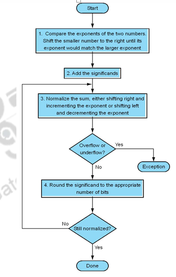
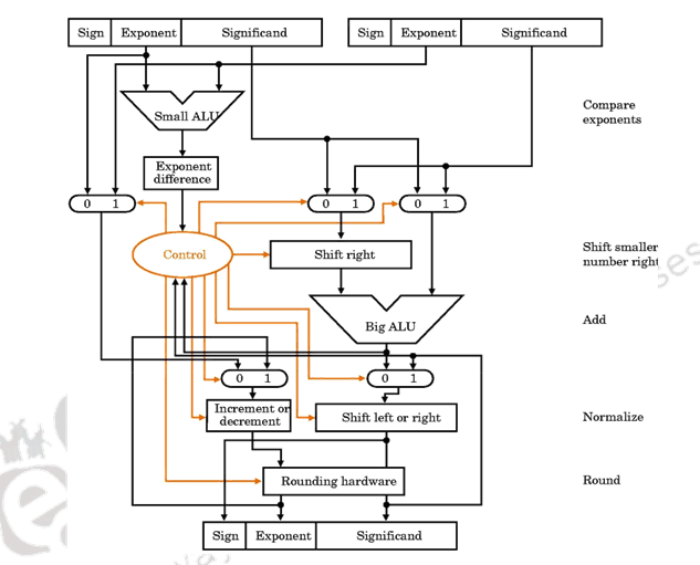
The organization of a floating point adder unit and the algorithm is given below.

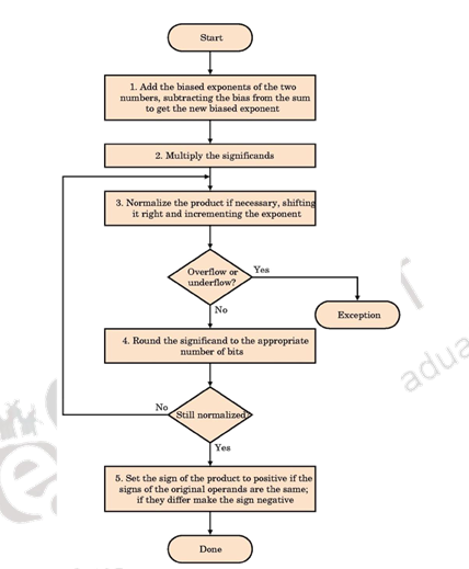
The floating point multiplication algorithm is given below. A similar algorithm based on the steps discussed before can be used for division.

Rounding

The floating point arithmetic operations discussed above may produce a result with more digits than can be represented in 1.M. In such cases, the result must be rounded to fit into the available number of M positions. The extra bits that are used in intermediate calculations to improve the precision of the result are called guard bits. It is only a tradeoff of hardware cost (keeping extra bits) and speed versus accumulated rounding error, because finally these extra bits have to be rounded off to conform to the IEEE standard.

Rounding Methods:

• Truncate

–   Remove all digits beyond those supported

–   1.00100 -> 1.00

• Round up to the next value

–   1.00100 -> 1.01

• Round down to the previous value

–   1.00100 -> 1.00

–   Differs from Truncate for negative numbers

• Round-to-nearest-even

–   Rounds to the even value (the one with an LSB of 0)

–   1.00100 -> 1.00

–   1.01100 -> 1.10

–   Produces zero average bias

–   Default mode

A product may have twice as many digits as the multiplier and multiplicand

–   1.11 x 1.01 = 10.0011

For round-to-nearest-even, we need to know the value to the right of the LSB (round bit) and whether any other digits to the right of the round digit are 1’s (the sticky bit is the OR of these digits). The IEEE standard requires the use of 3 extra bits of less significance than the 24 bits (of mantissa) implied in the single precision representation – guard bit, round bit and sticky bit. When a mantissa is to be shifted in order to align radix points, the bits that fall off the least significant end of the mantissa go into these extra bits (guard, round, and sticky bits). These bits can also be set by the normalization step in multiplication, and by extra bits of quotient (remainder) in division. The guard and round bits are just 2 extra bits of precision that are used in calculations. The sticky bit is an indication of what is/could be in lesser significant bits that are not kept. If a value of 1 ever is shifted into the sticky bit position, that sticky bit remains a 1 (“sticks” at 1), despite further shifts.

To summarize, in his module we have discussed the need for floating point numbers, the IEEE standard for representing floating point numbers, Floating point addition / subtraction, multiplication, division and the various rounding methods.

Web Links / Supporting Materials

• Computer Organization, Carl Hamacher, Zvonko Vranesic and Safwat Zaky, 5th.Edition, McGraw- Hill Higher Education, 2011.
• Computer Organization and Design – The Hardware / Software Interface, David A. Patterson and John L. Hennessy, 4th.Edition, Morgan Kaufmann, Elsevier, 2009.